From N-grams to CodeX (Part 1 - N-grams -> RNN)
Many language understanding tasks that were almost infeasible to solve only few years ago emerge as ready-to-use products nowadays. This series serves as an overview to language models, the cornerstone for almost all language tasks.
- N-gram to CodeX Series Introduction
- What is a language?
- Statistical Language Model
- Neural Networks for Language Modeling
- Language Modeling as a Sequential Prediction Problem (RNN)
- Generating Sequences From a Neural Language Model
- Conclusion
N-gram to CodeX Series Introduction
Language acquisition is one of the quintessential human traits. All normal humans speak, and no nonhuman animal does. Language enables us to know about each other’s thoughts, which is the foundation for human cooperation. Most natural languages structure are amazingly complex. Nevertheless, every child manages to learn it without no formal lessons.
Natural Language Processing (NLP) is currently one of the hottest research areas in AI. It achieved remarkable results in numerous tasks, varying from sentence sentiment analysis to conversational chatbots and code auto-completion. Many regard language understanding as the holy grail of AI and several benchmarks to test AI capabilities can be described as NLP tasks, such as the famous Turing test.
A crucial component in the exponential growth of NLP success was the use of deep learning. Tasks that were considered extremely difficult for decades are now almost obsolete using deep learning methods. In this series of blog posts, I will focus on a crucial milestone in this success story - language models. I will provide an overview of statistical language models, neural network-based language models, and some practical implementations that are being used today (such as code auto-completion by CodeX).
What is a language?
In a nutshell, the goal of NLP is to give the computer the ability to “understand” language. However, simply formulating what is a language to a computer seems to be a hard task for us. One might try to somehow capture the language structure, and somehow encode a complete set of rules that specify the correctness of each sentence. That also might be used to generate correct sentences. However, it is conceptually hard to disentangle the correctness of sentences from their meaning. Understanding language, in a way that humans do, intuitively consists of a deeper grasping of the meaning of words. Without it, how can the computer analyze the sentiment of text? That’s not merely a syntactic issue.
The prominent computational approaches that give some level of language understanding to computers nowadays are relying on statistical learning of a language model for large amounts of text.
Random thoughts on language learning While reading on that stuff, it became weird to me that I seek to understand how to “teach” language to a computer while I clearly have no clue about how human infants learn them. Are we biologically biased toward language? Why the ability to learn a language weaken with age? Maybe through the process of giving this ability to machines, we will gain intuition on our human brain mechanism.
Statistical Language Model
Language modeling is all about determining the probability of a sequence of words. For a sequence of length n, the language model assigns its probability.
\[\begin{equation} P(W_1,W_2,...,W_m) = \Pi_{i=1}^{m}{P(W_i|W_1,W_2,...,W_{i-1})} \end{equation}\]However, for long sequences that probability is computationally expensive to compute. A common assumption that is being used is the Markov assumption. The Markov assumption simply states that only some period of the sequence history influences the probability of the next word. Let’s refer to that period of history that affects the probability as the influence window. In the extreme case, history does not influence at all, and that influence window is empty. In that case, the language model boils down to simply modeling the probability of the current word:
\[\begin{equation} P(W_{i}|W_{1},...,W_{i-1}) \approx P(W_{i}) \end{equation}\]However, obviously, some part of the sequence history should be used to approximate the probability of the next word. The subset of the history that is being taken into consideration is called N-gram, where N is the history length. Generally, the N-gram language model approximation is computed as:
\[\begin{equation} P(W_1,W_2,...,W_m) \approx \Pi_{i=1}^{m}{P(W_{i}|W_{i-n-1},...,W_{i-1})} \end{equation}\]Practically, given a large-enough text corpus, computing these probabilities is as simple as counting. For a given word (W) to appear after some sequence (S), we need to find the ratio between the number of times that happened (S followed by W) and the number of times the sequence (S) appears at all. That can be expressed as:
\[\begin{equation} P(W_{i}|W_{i-n-1},...,W_{i-1}) \approx \frac{count(W_{i-n-1},...,W_{i-1},W_i)}{count(W_{i-n-1},...,W_{i-1})} \end{equation}\]The partition to different N-grams, for N=1,2,3, can be visualized as:
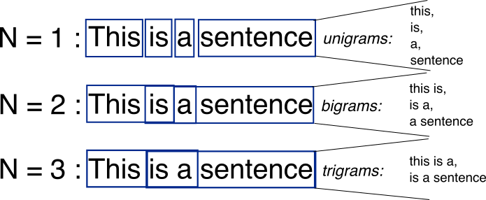
Example of N-gram for N=1,2,3. Image source.
Practical Issues of Statistical Language Models
That count-based approximation suffers from two main issues that need to be addressed for the practical usage of a statistical language model.
First, not all possible N-grams (assuming N=3 for now) appeared in the training corpus. For example, consider the sequence “Omri’s blog post”. What should be the value of the probability P(“post” | “Omri’s blog”)? Assuming “Omri’s blog post” is not in the corpus, the numerator in the equation above will be 0 and therefore the probability will be 0, which is clearly an underestimate if you read this post now. This is termed as the sparse data problem. I am skipping the various methods to solve that problem and refer you to read Goodman, 2001 for more details. Another fun read is from Brants et. al, 2007, where they outline Google’s large-language-model (which is simply a 5-gram LM!) solution for machine translation.
Another issue is the memory/space requirement of that language model. Consider a language with vocabulary with |W| words that we want to approximate with an N-gram language model. That means we need to somehow store the computed probability for every possible sequence. It basically means we need to store |W|^N values in some kind of probability table! In the first decade of the 2000s, when memory was relatively scarce, it took some heavy lifting of engineering from Google to simply be able to access and update this table, which weighed about 2TB.
Neural Networks for Language Modeling
Bengio et al., 2003 proposed a simple neural network to solve language modeling. They trained a network that took as input a sequence of (N-1) words and produced as output the probability for the next words in that sequence. They supervised it such that it will estimate a probability of 1 for the true next word (and thus, near 0 probability for other words). They used the following architecture for the network:
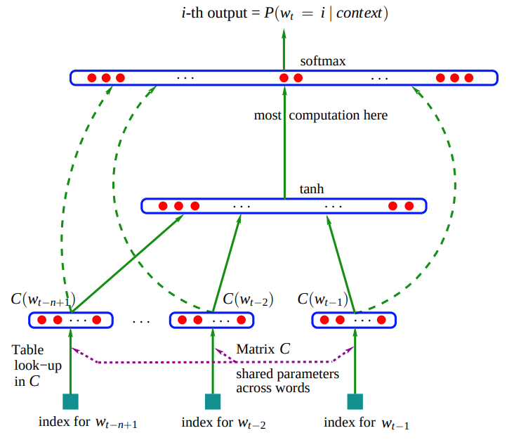
The neural network architecture proposed by Bengio et al., 2003. Image from paper.
The figure might look complicated, but it essentially contains three components that are still relevant, almost 20 years after this paper was published, in most modern neural language models:
- Embedding layer - A mapping from a word to a vector that represents it. They refer to it as “distributed feature vectors”, which is a |V|xH matrix where H is the dimension of the vector that represents a word, and |V| is the vocabulary size.
- Hidden layers - Layers that perform non-linear computation on the concatenation of the feature vectors from the embedding layer.
- Probability layer - Layer that produces a probability distribution over the words in the vocabulary V.
Note that the last layer outputs a probability distribution (using the softmax function). That means that we get some probability estimation for each word in the vocabulary to appear after the (N-1) sequence of words we gave the network as input. To supervise it, we want the network to predict the true word that appeared in the sequence. Therefore, we want to maximize the probability that the network will assign to the correct word. Indeed, Bengio et al. relied on this idea of maximizing the probability to supervise the network. This idea is referred to as Maximum Likelihood Estimation.
It is astonishing to observe the simplification that occurred over these last 20 years that enable them to implement and experiment with their paper’s proposed architecture. Their paper focuses on many technical details, such as the possible types to parallelize the training & inference on CPUs. However, today that can be run on a simple laptop machine and implemented with ~100 lines of Python code. A great example was recently published by Andrej Karpathy, where he implemented from scratch various language models. I highly recommend reading his code and specifically his implementation of Bengio et al. MLP.
Implementation note - Bengio et al. trained the network by maximizing the log-likelihood (i.e., using gradient ascent). In Karpathy’s implementation he is minimizing the cross-entropy loss. Recall that these two are equivalent in the case of hard labels (i.e., using one-hot vectors for ground truth, where only the index of the correct word is assigned 1 and all others are assigned 0 probability).
Regarding the discretized n-gram statistical models, note that their neural language model only scales linearly with |V|, in contrast to the exponential scaling of the n-gram model. Furthermore, Bengio et al. show a 24% performance increase in perplexity with respect to the best statistical n-gram model of his time.
Perplexity
How can one evaluate a language model? Recall that a language model provides a probability for the next word given a sequence. So for a natural sentence, we want our model to assign a high probability for each word given its preceding sequence. If we get high probabilities for all the sequences in our test set, then the language model “is not surprised” (not perplexed) by the test set. Without getting into the details, one can compute the perplexity by taking the exponent of the cross entropy loss. For the derivation, please read more. Intuitively, when evaluating a test set, the higher the probabilities assigned by the model, the lower the perplexity. Note that this metric is certainly not the only one being used and has several limitations, and we will return to that in future posts.
Mitigating the Computational Bottleneck of Neural Language Models (Hierarchical Softmax)
Recall that the last layer in our neural language model maps from the hidden layer size to the vocabulary size. In general, the vocabulary tends to be really big (10–50K words in vocabulary considered common). Computing the softmax on that layer is prohibitively expensive. Let’s recall what the softmax function does:
\[\begin{equation} p(w_i) = \frac{e^{z_i}}{\Sigma_j e^{z_j}}, z_i = V_i\cdot h \end{equation}\]The softmax function, p, computes the probability for the ith word. The \(z_i\) are the activations from the previous layer, and V is the weight matrix of the softmax layer.
Observe that to compute the denominator of the softmax, one needs to compute the dot product all for every word in the vocabulary (denoted as \(z_i\)). That is one of the main computational bottlenecks in training neural language models.
A possible solution is factoring this softmax into a hierarchical prediction problem. Instead of predicting the probability of the word given the context, predict the probability of a specific word category given the context, and the probability of the specific word given the category:
\[\begin{equation} P(w=w_i|seq) = P(C=c_k|seq)P(w=w_i|C=c_k, seq) \end{equation}\]The probability of the word \(w_i\) given sequence can be factored to the multiplication of the probability of the class \(c_k\) given the sequence by the probability of the ith word given the class \(c_k\) and the sequence.
That means we can break the softmax layer into multiple layers. In the naive solution, we break it into two layers. The first layer predicts the probabilities for each category, \(C_k\). That means we evaluate the softmax function on that layer output, which is on the size of the number of classes. Since we are using a two-layer solution, the first layer has \(\sqrt{ \lvert W \rvert }\) elements. Note that \(\lvert W \rvert\) denotes the number of words in the vocabulary.
Now for a given target word \(w_i\), we know which category it is contained in and need to only compute the probabilities of words in that category. That means we again evaluate the softmax function on the words in that specific category, which again have \(\sqrt{ \lvert W \rvert }\) elements. Instead of evaluating the softmax function for a |W|-dimension vector, we evaluated it on two \(\sqrt{ \lvert W \rvert }\)-dimension vectors. I highly recommend reading this code for an implementation of the two-layer Softmax in Pytorch.
Morin and Bengio, 2005 proposed to extend this idea to a binary tree. That essentially means that there will be \(\log (\lvert W \rvert )\) layers. Several other improvements to the hierarchical softmax proposed later, all rely on the property of factoring the probability to hierarchical prediction.
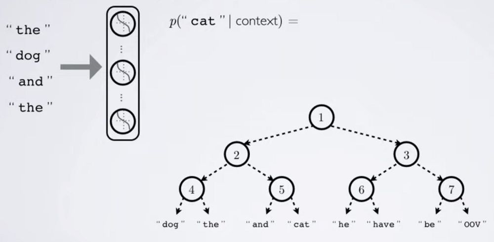
Illustration of the hierarchical softmax with binary tree proposed by Morin and Bengio, 2005. Image source.
Language Modeling as a Sequential Prediction Problem (RNN)
In Bengio et al., 2003 architecture the “temporal window” was pre-defined to some fixed size, analogous to the N-gram statistical models. However, that poses a limitation for the network to grasp relations that are longer than the window size (e.g., learning a 6-word relation is impossible with a 5-gram neural network). It is obvious to us humans that we exploit a much longer context. How can we give this ability to our model?
Intuitively, we would like to model some “memory” in the network that is updated over time and has the capacity to model long-term relations. Fortunately, that is what Recurrent Neural Networks (RNN) is all about, and it was used by Mikolov. et al., 2010 and Mikolov. et al., 2011 to build a Recurrent Neural Network Language Model (RNNLM).
There are many variants of recurrent architectures, and the authors used probably the simplest one. They add to the network a hidden state, denoted as h. For a given input word w at time t, they concat the input word (a one-hot vector) and the hidden state at time t-1.
\[\begin{equation} x(t) = [w(t),s(t-1)] \end{equation}\]The input x to the network at time t is a concatenation of the current word and the last hidden state.
Then, they feed this x(t) to a two-layer neural network and get a prediction (as a probability distribution) denoted as y(t). They save the hidden layer activation of this network in h(t) for future timesteps, which acts as memory. While training, the network is trained to minimize the cross entropy loss on y(t), as before. However, observe that now the length of history that the networks receive is not constant. Even if we were to use sequences of fixed size in the training set (i.e., 5-gram sequences), the network would try to predict the second word from the first, the third from the first two, and so on. Moreover, it will try to predict the first word given no history (hidden state set to zero)! That means that the network needs to somehow learn to attend to a non-fixed size history window, by maintaining an internal state. For more details on RNN, please read this survey.
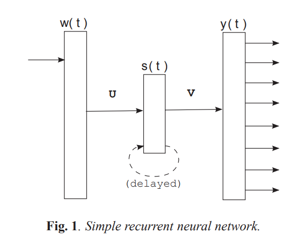
A simple recurrent neural network. w(t) is the input word, s(t) is the hidden state, and y(t) is the prediction, all at time t.
Using this simple recurrent model, Mikolov. et al. managed to gain a 50% reduction in perplexity. That was a motivating result for many researchers to find interesting ways to incorporate memory into neural networks in general, and specifically in neural language models.
RNN is Not Flawless
Although the RNN results were motivating, it was already well-known for years that training an RNN is notoriously hard. The main difficulty was the backpropagation of the error in long sequences. That is referred to as Back Propagation Through Time (BPTT).
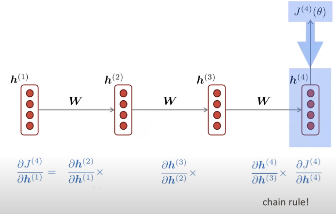
Illustrating the Back Propagation Through Time in training an RNN with a sequence of size 4. Image source.
In the above figure, the loss function is denoted as J, and the hidden vector that we are updating is h. Note that since we backpropagate through time, as the sequence becomes longer, the derivative is a product of more multiplications of derivatives (due to the chain rule). This introduces two potential problems:
- Vanishing gradients - If the intermediate derivatives (i.e., the elements we are multiplying) are smaller than 1, for a long sequence it will result in a really small number. That means that the gradient is decaying with time. Also recall that the gradient is computed with respect to all time steps, making the model learn only near-term effects.
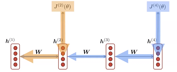
Note that h(1) gradient is computed from all timesteps. Since the gradient from the “far future” might vanish, the model will essentially learn only near-term effects. Image source.
- Exploding gradients - Similar to the above situation, but now consider the intermediate derivatives to be big (higher than 1). That might cause the gradient to be very big. Practically that means we’ll take gradient steps that are too big and fail to converge.
Solving the exploding gradients problem is relatively easy - just clip the gradient. Clipping the gradient is fine since we still take a step in the gradient direction, but just a smaller one. However, vanishing gradients is harder. Intuitively, one would like to ensure that the intermediate derivatives for long sequences are “nice” (ideally around 1). An RNN architecture that mitigates this problem was proposed by Hochreiter & Schmidhuber in 1997, called Long Short-Term Memory (LSTM). I highly recommend reading this post to understand LSTM in detail.
Using the LSTM architecture, Sundermeyer. et al., 2012 gained an 8% perplexity reduction compared to vanilla recurrent neural networks shown above.
Generating Sequences From a Neural Language Model
Now that we have a neural language model at hand, how can we sample sentences from it?
Note on tokenization - when training a network on textual data, the text usually is converted to tokens. Basically, the set of all possible tokens will be composed of the word vocoulary, with potential decomposition of words to sub-words (as splitting “reading” to “read” and “ing”). Moreover, special tokens (<sos> and <eos>) added to identify start and end of sequences. This allows the model to learn when a sentence ends, and what words are more probable in its beginning.
We wish to sample the most probable sequence given some prefix. The prefix can be a start of seqeunce (<sos>) token, or any sequence we want to continue generating from. That means we look for a sequence that maximizes the following probability:
\[\Pi_{i=1}^{N}{P(W_i|W_1,W_2,...,W_{i-1})}\]The naive answer is to feed the model the prefix and choose the next word that maximizes the predicted probability from the model. Then, feed this word to the network and iterate this step until the word you get is the end of sequence (<eos>) token. That approach is the greedy approach to generating sequences.
\[\operatorname{argmax}_W P(W|W_1,W_2,...,W_{i-1})\]The greedy approach chooses the word that maximizes the probability at every step.
However, the greedy approach does not gaurantee to sample the most probable sequence. Please read here to understand why.
Ideally, we would check the probability for every possible sequence, and return the sequence with the highest probability. That will obviously give us the sequence we look for, but it is computationally infeasible. Therefore, the Beam Search algorithm is most commonly used. Essentialy, beam search keeps track at each timestep on K sequences (K is a hyperparameter) with the highest probability (instead of only a single sequence in the greedy approach, and \(\lvert V^ N \lvert\) sequences in the ideal approach, where \(\lvert V \lvert\) is the vocabulary size and N is the maximal sequence length). Based on these K sequences, it assigns them to the language model and searches for the next K sequences with highest probability. I refer the reader to read more on beam search here.
Conclusion
We learned about statistical language models, their limitations, and the strength of neural network-based architectures. Then, we learned about RNNs, and their challenges and finished by understanding how to sample sentences from neural language models.
In Part 2, we will focus on the limitations of the RNN (and LSTM) architecture and describe the attention mechanism as a solution to them. Then, we will discuss self-attention, the main building block of the famous Transformer architecture. Later in this series, we will discuss modern large language models (LLM) and some applications (code auto-completion).