Neural Implicit Representations for 3D Shapes and Scenes
In recent years there is an explosion of neural implicit representations that helps solve computer graphic tasks. In this post, I focus on their applicability to three different tasks - shape representation, novel view synthesis, and image-based 3D reconstruction.
- Introduction
- A Brief Background on Computer Graphics
- NNs for shape representation
- NNs for scene representation
- NNs for understanding scenes
- Make it faster
- Conclusion
Introduction
The field of computer graphics has flourished in recent years alongside deep learning, with several contributions that have had a major impact on the field. Computer graphics tackles the problem of creating images with a computer. While it might sound simple, it is certainly a complex task to create physically correct and realistic images. To do so, one needs to understand how to represent 3D scenes, which typically contain light, different materials, several geometries, and the model of a camera that is taking the picture. Fortunately, researchers have found fascinating ways to solve computer graphics problems using deep learning models.
To put it simply-but-not-accurate, this post aims to distill the progress of the following deep learning-based solutions to computer graphics tasks:
-
2017–2019 - How to represent shapes with neural networks (NN)? I will focus on the line of works that used Signed Distance Functions to do so.
-
2019–2020 - How to represent scenes with NNs? Specifically, how can a neural network represent a full scene, with all its fine-grained details from lightning, texture & shapes?
-
2021 - 2022 - How can we understand scenes with NNs? Specifically, Given the neural scene representation, how can we reconstruct the 3D surfaces in the scene?
-
2022 - How can we make it faster?
This is simply my way to distill the progress into different stages, while obviously, the field did not progress in such a clear way. People tried to understand scenes with NNs before 2021, and shape representation is still something people are working on (generalizing between shapes is still an issue). However, this order makes the ideas and works I’ll cover in this post, in my opinion, easier to grasp.
A Brief Background on Computer Graphics
While I assume the reader to be familiar with deep learning (gradient descent, neural networks, etc.), I will give here a brief background for some of the terms that will be used in this post for completeness.
Ray-tracing vs rasterization for rendering
Note that there are two categories for rendering images - rasterization and ray-tracing. Check this post from Nvidia for an intro to them, and I highly recommend watching the videos from Disney on Hyperion, their (ray-tracing) rendering engine, that explains intuitively the process of computationally modeling the paths of light from the light source, through several collisions with objects, to the camera. However, if you’re not that familiar with rendering, just note that rasterization is much faster on modern GPUs, yet it does not model the physical world as well as ray-tracing-based rendering. In this post, I will focus on works that leverage differential ray-tracing rendering as they tend to produce superior results, and I will describe ways to make them usable for real-time applications.
3D Geometry Representations
While it is clear that a 3D scene contains several 3D objects, it is not clear how to represent their geometries. There is no canonical representation that is both computationally and memory efficient yet allows for representing high-resolution geometry of arbitrary topology. Several representations evolved, and the most commonly used are meshes, voxel-based or point-based. If you are not familiar with those terms, I refer you to read them before following on. However, the important thing to note is that those approaches have inherent tradeoffs regarding efficiency (voxel-based representations memory usage grows cubically with respect to the resolution), expressivity (fine geometry such as hair is notoriously hard to model using meshes), or topological constraints (producing a watertight surface, i.e. a closed surface with no holes in it, directly from a point cloud may not be a trivial task).
All the representations above share a common property - they rely on an explicit formulation of the geometry. However, it does so by approximating the 3D surface with discrete objects, such as triangles, grids, or simply points. Another common way to represent 3D objects is using continuous implicit representations. Generally, an implicit function represents a geometry as a function that operates on a 3D point that satisfies:
- F(x,y,z)<0 - interior point
- F(x,y,z)>0 - exterior point
- F(x,y,z)=0 - surface point
Specifically, the Signed Distance Function (SDF) satisfies those properties. The SDF is simply the distance of a given point to the object boundary and sets the sign of the distance accordingly to the rules above. If implicit representations are new to you, I recommend reading the lecture notes from the Missouri CS8620 course. Keep in mind that the SDF has many nice properties (can be used to calculate intersections easily and make ray-casting fast). However, it is not trivial how to obtain the SDF of some shape?
Visually, an SDF of a sphere can be seen as:
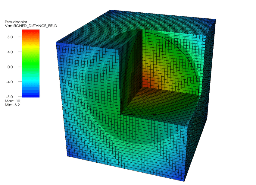
A visual of a signed distance surrounding a sphere. Figure source.
Computer Graphics Tasks
Recall that the general goal of computer graphics is to create images using computers. This goal can be decomposed into several problems. Today, I will focus on how deep learning helps solve the following computer tasks:
- Shape Representation - As I detailed above, representing 3D shapes is not trivial. While several classical representations exist, I will detail in this post how using neural networks allows us to represent continuous 3D shapes (the SDF specifically) efficiently.
- Novel View Synthesis (NVS) - Given several images from a scene, how can we generate images from new views? How many images are needed, and what properties other than the view can we control (i.e., can we generate views with different lighting)?
- Surface Reconstruction - Given several images of a surface, how can we reconstruct its 3D model?
One might now wonder if doesn’t solve NVS implicitly solves the surface reconstruction task? It is reasonable to think that if a computer can generate novel views of a scene, it had to (implicitly) reconstruct the 3D model of the scene. Therefore, it might seem like solving NVS (i.e., fitting a NeRF to a scene) solves the surface reconstruction problem. While it sounds correct, it is not entirely true and I will describe a mechanism that reconstructs a surface by solving the NVS task.
NNs for shape representation
How can one obtain an efficient and compact representation while capturing high-frequency, local detail is a challenging task. While implicit representations are an efficient way to represent shapes, it is hard to obtain them using classical methods. Among the first successful applications of deep learning for this task, was DeepSDF.
DeepSDF - Neural networks to represent the SDF
Given a mesh, how can we find its SDF? Classical approaches approximated an SDF by discretizing space by a 3D grid, where each voxel represents a distance. These voxels are expensive in memory, especially when a fine-grained approximation is needed.
DeepSDF suggested approximating it using a neural network, that simply learns to predict for a given point its SDF value. To train the network, they sampled a large number of points with their corresponding SDF. They sampled more points around the object’s surface to capture a detailed representation.
Once we can represent the SDF using a neural network, several questions about this representation arise. Can one network generalize to represent several shapes, instead of training a specific network for each shape? If so, does the continuous representation of multiple shapes enable us to interpolate between them? Without diving into the details, I note that DeepSDF indeed showed some level of generalization between shapes, by conditioning the DeepSDF network on a trainable shape code. Please refer to DeepSDF Section 4 for more details.
DeepLS - Trading computation for memory
While DeepSDF achieved remarkably good results in approximating the SDF, it was costly to train and infer from. The MLP network typically was built from ~2M parameters, making the training & inference for a high-resolution 3D shape to be costly. Recall that DeepSDF is a coordinate-based (i.e., a network that operates on a single coordinate at a time) network. Therefore, during training, a gradient for each one of the ~2M parameters has to be computed for every single point. Training DeepSDF for a specific mesh was done with 300–500K points, and that caused the training to be computationally expensive. Accordingly, using the network for inference was costly as well.
A naive suggestion is to make the training & inference of DeepSDF faster by simply using a smaller network. However, as shown by DeepSDF, their network architecture was chosen after considering the speed vs accuracy tradeoff, as they found that a smaller model performs worse. A more sophisticated approach is needed.
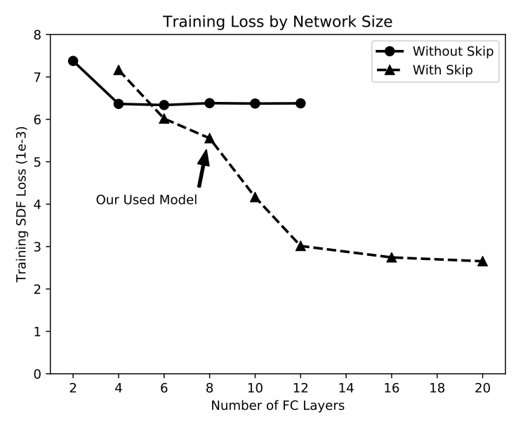
DeepSDF regression accuracy as a function of network depth. Figure from DeepSDF.
DeepLS suggested solving it by incorporating a crucial and well-known observation in the classical computer graphics literature - A large surface can be decomposed into local shapes. Therefore, they divide space into a grid of voxels, where each voxel stores information about the surface in a small local neighborhood. This information is stored as a learned latent code (i.e., A latent code \(z_i\) is stored for each voxel \(V_i\)). That way, the grid essentially encodes local information about the shape, and the network maps this local information to the SDF value. In essence, their method is:
- Divide space into a regular grid of voxels.
- For a given point \(x\) find the corresponding voxel on the grid \(V_i\).
- Transform \(x\) to the voxel \(V_i\) local coordinate system, \(T_i(x) = x-x_i\).
- Feed the latent code \(z_i\) of the voxel \(V_i\) and the transformed coordinate \(T_i\) to the network and regress the SDF.
- Repeat 2–5 for some large number of steps, while optimizing for the latent codes \(z_i\) and the neural network parameters.
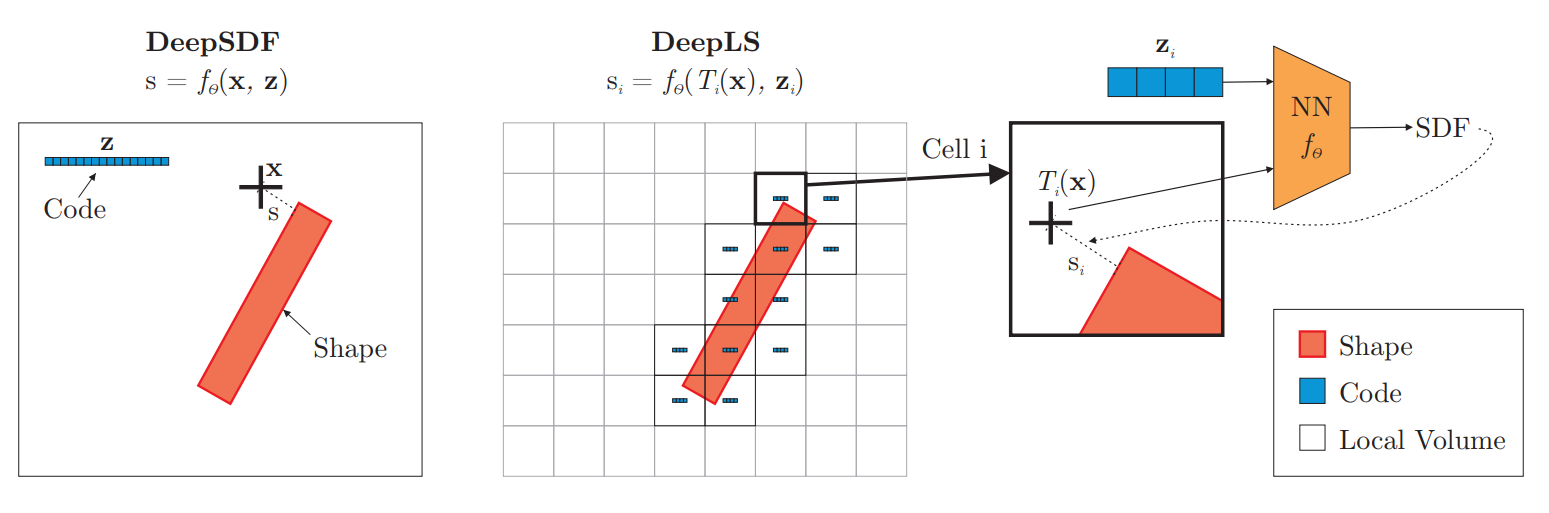
A 2D comparison of DeepSDF and DeepLS approaches. DeepSDF represents a specific shape SDF using a point and some shape-code (z), while DeepLS utilize a grid to represent local shape codes. Note that DeepLS optimizes both the neural network parameters and the latent vectors \(z_i\). The figure is taken from DeepLS
Here I suggest another way to think about their suggestion. A common theme in analyzing learning problems is to split the task into two different sub-tasks. First, a feature extraction task, which given the raw data (a 3D point, in our case) produces an extracted feature vector that describes the data. Then, a second sub-task is to regress the SDF value given that feature vector. Traditionally, the feature extraction part does the “heavy lifting” of transforming raw data into good representation features that enables the regression (down-stream task, in general) to be simple. While this description might sound vague, today’s deep learning practitioners are used to the idea of using a large frozen (already trained on a massive dataset) neural network as a feature extractor and training a small model that takes these features as input for a given task.
With this in mind, I see the DeepLS’s grid as a local feature extractor and the neural network as a simple regression model. Therefore, the regression model can be much smaller. Specifically, their neural network has only 50K parameters, in contrast to the ~2M parameters of DeepSDF. Moreover, while the grid itself might be large (even larger than the DeepSDF network itself), at each pass through the network only a small amount of parameters affect the computation! That causes the training and inference to be much faster, while trading compute for memory.
Overall, using the grid, DeepLS is significantly more efficient than DeepSDF. In the following example, DeepLS is 10,000x faster to train than DeepLS.
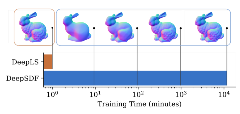
DeepLS and DeepSDF training time comparison on the Stanford Bunny. DeepSDF took 8 days to reach DeepLS results after 1 minute. That’s about 10,000x faster. Figure from DeepLS.
Note that DeepLS measured their contribution in several aspects, while I focus only on efficiency. Please refer to their paper for more details.
NNs for scene representation
In this part, I will focus on the scene representation task. Specifically, on solving the novel view synthesis task using neural networks, as suggested by SRN and NeRF. This might not seem very related to the previous part at first, but in the next part, it will hopefully make sense.
SRN - Representing Scenes With Neural Networks
Until now, we discussed shape representation. However, to solve the novel view synthesis task, a scene representation is needed. Ideally, this representation will be continuous and enable one to query the scene from different views and control the scene properties (for example, its light sources). SRN proposed to represent the scene using a neural network.
Wait, how can we train a neural network to represent the scene? For us to do so, we need to somehow supervise the network on how well it represents the scene. It means that we need it to generate images from specific views we have on the scene and train it to minimize the difference between the generated image and the true one. While generating images using neural networks (so-called generative models, such as the famous StyleGAN) made great success in recent years, it failed to do so in a multi-view consistent manner, and precisely conditioning it on a 3D viewpoint is non-trivial.
Therefore, SRN suggested using a differentiable renderer to train a network to represent the scene. While the SRN training mechanism is somewhat complex, the general idea can be intuitively simplified. Given a 3D coordinate, the neural network represents it as a feature of the scene at that coordinate. Then, they generate the corresponding pixel color for that coordinate’s features, using a differentiable renderer. For a given a specific pixel, its color is affected by multiple 3D coordinates along the ray reaching the camera and intersecting that pixel. The ray from the camera through the pixel can be seen in the figure below.
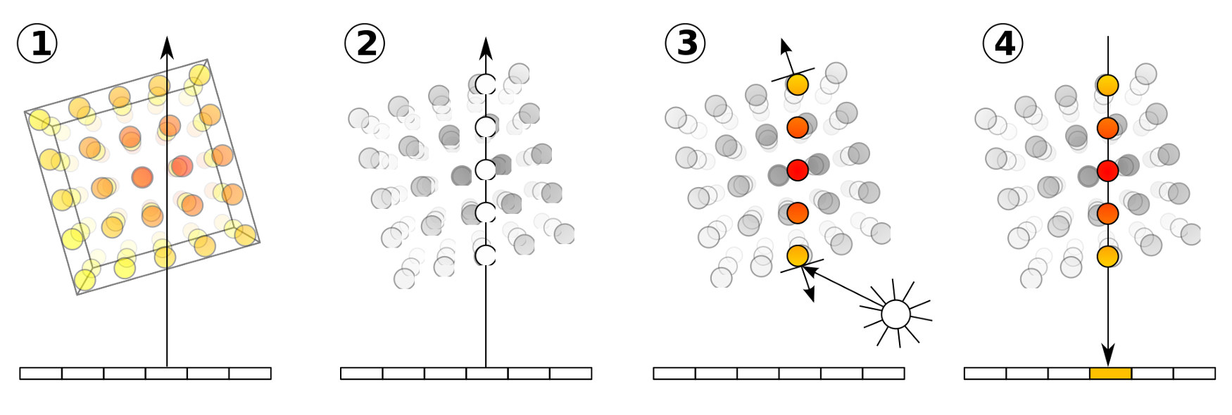
The four basic steps of volume ray casting. For each pixel in the image plane (the bar at the bottom of the image) a ray is marched through the volume (1). Several coordinates are sampled along that ray (2), and their colors are computed (3). Then, an aggregation of their colors defines the pixel color. Figure from Wikipedia.
However, since there are infinite 3D coordinates along that ray, and the scene geometry implicitly emerges during training, SRN had to deal with a critical problem - how to decide what points to sample along the ray? Naively sampling an immense number of 3D coordinates for each ray without knowing where to focus is impractical.
Therefore, SRN suggested a somewhat complex temporal ray marching layer (called ray-marching LSTM) to solve the sampling problem. Specifically, they used an LSTM that given a ray starting for the camera, iteratively looks for its intersection 3D coordinate with the scene geometry and returns that 3D coordinate extracted features. Then, a pixel generator network is used to map the 3D coordinate feature vector to a single RGB value - the corresponding pixel color. By doing so, they compare the color of the generated pixel and the original pixel color from the given image, thus supervising the scene representation network using images only.
While their mechanism is somewhat complex, I suggest you keep in mind the general flow of neural representation learning, as it is much simpler to grasp. Basically, given a set of images of a scene, we use a neural network to represent the scene and render that scene from different views, by simply supervising the network to produce views of the scene that are the same as the original views.
A crucial limitation that was acknowledged as possible future work in SRN’s original paper is modeling view and lightning effects. How one should encode this information to SRN was unclear.
NeRF - Neural Radiance Fields
As often occurs in research, simpler solutions tend to arise after complex solutions are suggested, yielding superior results with a more intuitive mechanism. The NeRF authors suggested modeling the scene using a (coordinate-based) MLP, that given a 5D input (a location and viewing direction) produces the color and density (RGB-alpha). Instead of mapping a coordinate to latent features, and using the complex mechanism of SRN to generate the corresponding pixel colors, NeRF directly regresses the RGB-alpha value for that coordinate and feeds it into a differentiable ray-marching renderer.
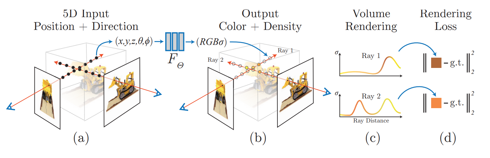
NeRF synthesizes images by sampling 5D coordinates (location and viewing direction) along camera rays (a), feeding those locations into an MLP to produce a color and volume density (b), and using volume rendering techniques to composite these values into an image (c). Figure from NeRF paper.
Volume rendering might sound scary. But the important thing to note is that volume rendering is basically all about approximating the summed light radiance along the ray reaching the camera. Since we are summing light, it is crucial that we can weigh “how much the light coming from some position along the ray coordinate affects the total light?” concerning the scene properties (occlusions, material, etc.). Intuitively, we would want to give large weight to opaque objects, and small weight to transparent objects, for us to be able to see through glass but not through tables. And that’s the crucial rule that predicting the density (sigma) value has in the NeRF algorithm.
Using the 5D coordinate-based MLP, NeRF estimates each pixel color by computing:
\[\begin{equation} \hat{C}(r) = \sum_{i = 1}^{N}T_i(1-exp(-\sigma_{i}\delta_{i}))c_i \end{equation}\]where \(T_i = exp(-\sum_{j = 1}^{i-1}\sigma_{j}\delta_{j})\). The predicted color of a ray traced from the camera through a pixel denoted as \(\hat{C}(r)\). Note that \(T_i\) computes the accumulated transmittance (i.e., the probability that a ray travels up to some distance without hitting an opaque particle). \(\sigma_{i}\) denotes the predicted density (alpha) value at a given 5D coordinate, and \(\delta_{i}\) is the distance between adjacent samples along the ray, which might not be equal between all samples due to non-uniform sampling.
I am skipping the specific parts, such as details about NeRF training mechanism, sampling coordinates along the ray, and positional encoding since a lot has been written on it before.
NNs for understanding scenes
NeRF suggested an amazingly powerful scene representation. Yet, it couples all scene properties together, from structure to lightning. Here, I’ll describe ways to extract a geometry (surface) out of it.
VolSDF & NeuS - From Density to Signed Distance
NeRF showed great success in capturing a scene. Yet, while NeRF can generate novel views of the scene, it is not clear how to extract the geometry. At first, it might sound trivial - we already predicting a density value for each coordinate, and that should vaguely describe a surface! Indeed, the density value is high around surfaces, and low far from them. However, defining the threshold for “high” density is far from a trivial task. Also, it is view-dependent, which is not a desired property for a geometry. Therefore, researchers looked for creative ways to modify the NeRF architecture by explicitly learning geometry.
Recall that an intuitive continuous geometry representation for deep learning is the SDF. Hopefully, we can train a NeRF to predict an SDF value and still use volumetric rendering to train it all end-to-end (and get supervision from the scene images directly, thus reconstructing the geometry without any 3D supervision!). Luckily, at NeurIPS 2021, two interesting papers tackled that specific problem. Their works are dubbed VolSDF and NeuS (read as “news”).
Both of them suggest training 2 networks -an SDF network, and a color/appearance network. They differ in the way they suggest transforming the SDF values to density values and using them in volume rendering. The main idea is as simple as that - we want to transform the SDF values such that points near the surface will receive high alpha values, and points far from it will receive low alpha values. That way, the colors of near-surface points will have the largest effect on the ray’s integral. The SDF to density transformation must satisfy the following properties, as described by NeuS:
- Unbiased - for a given ray, at points where the SDF function produces 0 (i.e., points on the surface) the density value should attain a locally maximal value. Note that we only desire locally maximal and not globally since there might be several surface intersections along the ray.
- Occlusion-aware - When two points have the same SDF value, the point nearer to the camera should have a larger contribution to the final output color.
Intuitively, the transformation is simply using the logistic distribution centered at zero to map SDF values to density values. This is convenient as it is a bell-shaped distribution that is centered at 0, thus assigning the largest density to the SDF value of 0, and decreasing density to SDF values elsewhere in a decreasing manner.
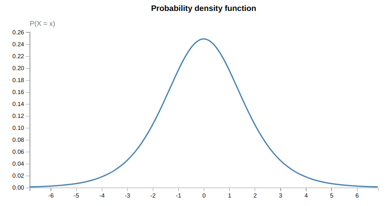
The PDF of the logistic density distribution with mean 0 and std 1. Naively, one can use this distribution to map SDF values to density values. However, as shown by NeuS and VolSDF, more sophisticated approaches are needed to make the transformation unbiased and occlusion-aware.
I refer the reader to the papers to read about the more sophisticated approaches to constructing the transformation from SDF to density values. While they both suggested a neat way to learn the SDF directly from scene observations, they are still left with a crucial limitation - training & inferring from these relatively large coordinate-based MLPs is still very slow. Specifically, training each one of them for a specific scene takes ~12–14 hours.
Make it faster
InstantNGP - Better memory vs compute tradeoff
There are two possible directions to make the training & inference of NeRF-based methods faster: sampling fewer points along each ray, or sampling faster. There are interesting ideas for sampling fewer points, but here I focus on sampling faster.
Recall that DeepLS made the sampling at DeepSDF faster by incorporating a learnable voxel grid. However, it traded the sampling efficiency with expensive memory costs, as the memory grows cubically with respect to the grid. How expensive? For a simple grid of size 128 with 16-dimensional latent vectors, one would need to store ~33.6M grid parameters, regardless of the MLP size (which is typically small, about 100–300K params). Unfortunately, simply making that grid smaller will have a severe impact on the performance and the ability to capture fine-detailed geometry. A better solution is needed.
Luckily, earlier this year InstantNGP suggested significantly decreasing the memory usage by replacing the grid with a multi-resolution hash grid. The key idea behind InstantNGP is to capture the coarse and fine details by several grids of different sizes. A low-resolution grid takes only a small amount of memory and captures coarse details only. A high-resolution grid may capture fine details, at the cost of tremendous memory usage. Therefore, they suggest indexing the high-resolution grids with a hash table. Traditionally, in computer science, hash tables are used to tradeoff computation time and memory usage. Their method goes as follows:
- Divide space into several grids of different resolution levels (coarse to fine grids).
- For a given point, x, find the indices of the corners of the containing voxels at each resolution level.
- Using the hash table for each resolution level, look up the feature vector of the corners.
- Trilinearly interpolate the feature vectors at each resolution level.
- Concatenate the vectors from each resolution level and feed them into the neural network.
- Repeat 2–5 for a large number of steps, while optimizing for the feature vectors at the multi-resolution grid and the neural network parameters.
This process is summarized in the following figure:
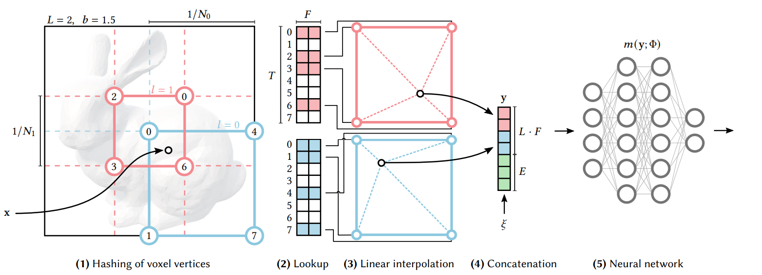
InstantNGP multi-resolution hash-grid demonstration in 2D. Given a coordinate x, find the enclosing voxels at each resolution (denoted as red and blue) and interpolate their edges. Concat the multi-res interpolated vectors and feed them into a neural network, and perform your desired coordinate-based task. Figure from InstantNGP.
However, it is crucial to point out an unintuitive issue regarding InstantNGP. When one uses a hash table, he needs to address the possibility of collisions (i.e., two different 3D coordinates that are mapped to the same feature vector) and how to resolve such collisions. Traditional computer science literature on this subject is filled with many sophisticated mechanisms and tricks to reduce the possibility of collision and find ways to quickly resolve collisions when they occur. However, InstantNGP simply relies on the neural network to learn to disambiguate hash collisions itself.
Note that InstantNGP provides a general recipe to train coordinate-based neural networks efficiently. Specifically, they show how effective their method is for NeRF, as well as for several other tasks not discussed here. To understand how effective their method is, note that the training time of a NeRF network for a single scene was reduced from ~12 hours to about 5 seconds. That’s about ~8500x faster in about 2 years.
MonoSDF - surface reconstruction with volumetric rendering, faster!
We learned how to modify NeRF training mechanism to enable explicit SDF representation learning. Also, we learned how to make the NeRF training & inference much faster by incorporating multi-resolution hash tables. MonoSDF combines both approaches along with geometric cues to make the surface reconstruction from posed images faster and more accurate.
Note that MonoSDF not only makes it faster but it aims to perform better, as it provides the network with geometric cues. Specifically, using advances in the field of monocular geometry prediction (i.e., predicting normal or depth images directly from a single RGB image), it supervises the network to render depth and normal images alongside the reconstructed monocular image for the NeRF training. These geometric cues improve both the reconstruction quality and the optimization time. Their (high-level) architecture is:
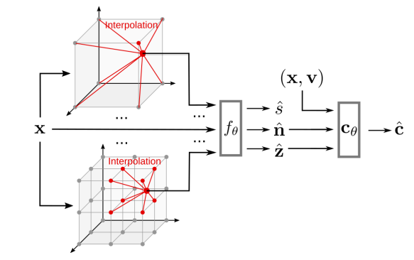
MonoSDF uses a multi-resolution feature grid (as in InstantNGP) to predict both the SDF value, normal (n), and depth (z) value for a given coordinate. They use volume rendering to reconstruct the scene and supervise with pre-trained networks that predict the depth and normal images. Figure from MonoSDF.
Conclusion
In recent years there is an explosion of neural implicit representations that helps solve computer graphic tasks. In this post, I focused on their applicability to three different tasks - shape representation, novel view synthesis, and image-based 3D reconstruction.
Having a neural representation is an enabler to solving many interesting tasks, but there is still a large space for improvement. We need representations that are editable (with explicit control), scalable (not only to small scenes in controlled environments), fast-to-query, and generalizable. Each of those requirements encompasses many challenges. I hope that in the following years I will look back on this post and be amazed by how the research community, once again, took us so far from what today seems almost unbelievable progress.