Many language understanding tasks that were almost infeasible to solve only few years ago emerge as ready-to-use products nowadays. This series serves as an overview to language models, the cornerstone for almost all language tasks.

N-gram to CodeX Series Introduction

Language acquisition is one of the quintessential human traits. All normal humans speak, and no nonhuman animal does. Language enables us to know about each other’s thoughts, which is the foundation for human cooperation. Most natural languages structure are amazingly complex. Nevertheless, every child manages to learn it without no formal lessons.

Natural Language Processing (NLP) is currently one of the hottest research areas in AI. It achieved remarkable results in numerous tasks, varying from sentence sentiment analysis to conversational chatbots and code auto-completion. Many regard language understanding as the holy grail of AI and several benchmarks to test AI capabilities can be described as NLP tasks, such as the famous Turing test.

A crucial component in the exponential growth of NLP success was the use of deep learning. Tasks that were considered extremely difficult for decades are now almost obsolete using deep learning methods. In this series of blog posts, I will focus on a crucial milestone in this success story - language models. I will provide an overview of statistical language models, neural network-based language models, and some practical implementations that are being used today (such as code auto-completion by CodeX).

Machine Translation Problem

今天，我们的故事从机器翻译说起. What does that Chinese sentence say? Luckily, we can use tools like Google Translate to tell that it says: “Today, our story starts with Machine Translation.”

How can we make a computer to translate sentences between languages? Specifically, assuming we have pairs (X, Y) of translated sentences between two languages, the translation problem can be expressed as a conditional probability. How can we approximate this conditional probability?

\[\large \begin{equation} P(y_1,...,y_{T_y}|x_1,...x_{T_x}) = \Pi_{i=1}^{T_y}P(y_t|x_1,...x_{T_x},y_1,..,y_{t-1}) \end{equation}\]

The conditional probability for the sequence Y given the sequence X. Note that the Y sequence has length $T_y$ and the X sequence has length $T_x$, which in general is not equal.

The conditional probability for the sequence Y given the sequence X. Note that the Y sequence has length T_y and the X sequence has length T_x, which in general is not equal.Inspired by the success of RNN-based methods in language modeling, researchers tried to use RNN for machine translation as well. However, it is not intuitive how to use RNNs to model the above conditional probability. RNN assumes a fixed length input-output mapping. In other words, referring to the above equation, it assumes $T_x$ is equal to $T_y$. That is not the case in machine translation, since the length of the sentence across languages is not fixed.

Encoder-Decoder RNNs

Cho et al., 2014 suggested solving the above problems by using two different RNNs for encoding the input sequence and decoding to the target sequence. The encoding RNN sequentially reads the input sequence and updates its internal hidden state (recall that an RNN maintains a hidden state that is updated every timestep). We now refer to this final hidden state as a context-vector c. The idea is that c now encodes all information needed to translate the input sequence, abstracting away its length and word positions, thus solving the abovementioned problems.

Using that context vector, they generate a sequence with the decoding RNN. The decoding RNN task is to model the probability:

\[\large \begin{equation} P(y_1,...,y_{T_y}|x_1,...x_{T_x}) = \Pi_{i=1}^{T_y}P(y_t|c,y_1,..,y_{t-1}) \end{equation}\]

The decoding RNN models the target sequence probability, conditioned on the context-vector c.

The decoding RNN can be thought of as a conditioned language model. If we ignore the conditioning on the context-vector c, this is simply a language model as we’ve seen in the previous part. Adding the context vector actually guides the language model to generate a specific sentence that is encoded in c.

General form

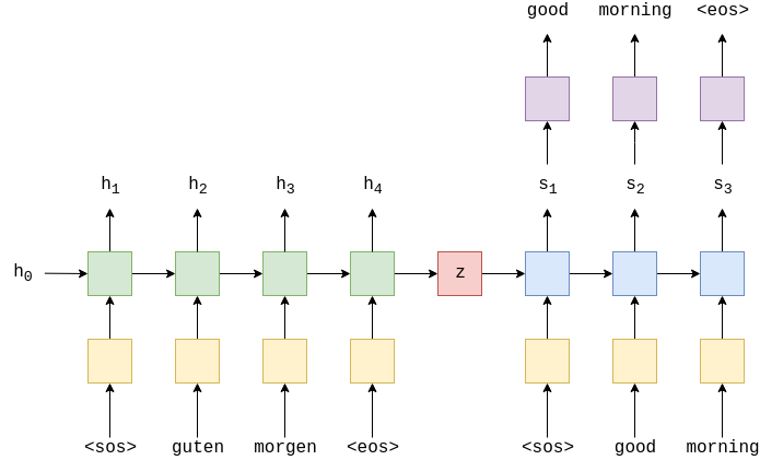
The general method of an encoder-decoder Neural Machine Translation (NMT) architecture. The green part is the encoder RNN, and the blue ones are the decoder RNN. Note that z is equal to h4, and the <sos>, <eos> tokens denote the start and end of the sequence, correspondingly. Image source.

Seq2Seq

Following this paper, the famous seq2seq paper was released by Sustkever et al., 2014. They used LSTMs and not “vanilla” RNN and outperformed the network. I highly recommend going over this amazing notebook that builds seq2seq LSTM-based model in PyTorch.

Solving the Encoder-Decoder Information Bottleneck with Attention

The encoder-decoder architecture has a critical assumption underlying it - all the relevant information to translate the sentence will appear in the last hidden state. Recall that compressing all the input sequences to a single vector helped us mitigate the problem of different input-output sequence lengths. However, observe that regardless of the sequence length, the context vector remains of the same size. It was only 3 months after the publication of the abovementioned encoder-decoder paper by Cho et al. 2014, that the same group released a paper that details the problem of this method with long sequences.

General form

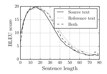
The BLEU score of the RNN encoder-decoder with respect to sentence length (both the source and reference lengths are shown). Clearly, the performance degrades drastically as the sentence gets longer. Image from Cho et al., 2014(b).

The BLEU score is a metric for the quality of translated sentences from the model. Intuitively, the closer the predicted sentence is to the human-generated target sentence, the higher the BLEU score it gets.

A better mechanism to pass the information from the encoder to the decoder was needed. Bahdanau et al., 2015 proposed the attention mechanism, which revolutionized the field. To explain their idea intuitively, I am omitting the usage of the bidirectional LSTM layer, as I find it not critical for understanding the attention mechanism.

The basic idea is to let the decoder network examine all the input sequences and extract the relevant information for the generation of each specific word in the output sequence. That is in contrast with the previous method that passed the decoder a single context vector that should serve all the words in the output sequence.

Recall that the encoder-decoder method regarded the last hidden vector of the input sequence as the context vector. Ideally, we would pass all the hidden vectors to the decoder, as they contain all the encoded information. However, doing so will return back the problem of different input-output length mappings, which the usage of a context vector solved.

Therefore, the attention solution is to compute a different context vector for each timestamp of the decoder. Let us define H and S as the vectors of hidden states produced by the RNNs across all timestamps:

General form

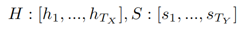
H is the vector of all hidden states from the encoder network. Recall that $T_x$ is the length of the input sequence. Similarly, S is the vector of all hidden states from the decoder network, and $T_y$ is the length of the output sequence.

The idea is to give each element of H a weight that describes how it affects the currently translated word in the output sequence. These weights for each couple of (input position, output position) are called attention weights. Intuitively, the name suggests that the weight tells the decoder where to put his attention on different parts of the input sequence.

How do we find the attention weights for each (input position, output position) couple? Let us change the notation and focus on finding an attention weight for couples of ($H_j$, $S_i$), according to the above definition of H and S. Essentially, two properties we want these attention weights to hold are:

For each couple (H_j, S_i), if the j-th input word should influence the translation of the i-th output word, the weight should be high. This is consOtherwise, it should be low. This is denoted as the alignment score. This will make sure that we extract only the relevant information for the translation of each output word.
We wish the attention weights to be a proper distribution over the vector H (i.e., the attention weights over the input for every timestamp should sum to one). This is achieved using softmax normalization.

Defining a function that computes the alignment is tricky and can be done in many ways, as we shall see later. The function that Bahdanau et al., 2015 defined is illustrated below. They trained a small neural network (as a part of the translation task, along with the encoder and decoder networks) to learn the mapping from a couple of ($H_j$, $S_i$) to a scoring value.

General form

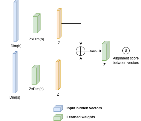
Given two vectors (h,s), Bahdanau et al., 2015 learned a mapping to a scalar score between them. This is referred to as the alignment score. Source: myself.

The mathematical definition of computing the alignment score $s_{ij}$ between two input and output positions can be expressed as:

\[\large \begin{equation} s_{i,j} = v_a^T tanh(W_as_i + U_ah_j) \end{equation}\]

$W_a$, $U_a$, and $v_a$ are learned matrices.

To get a proper probability distribution (satisfying the second property above), we pass the alignment scores of all input positions for a given output position through a softmax to get a probability distribution over the input sequence. This results in attention weights. Specifically, the attention weights for the i-th output position are:

General form

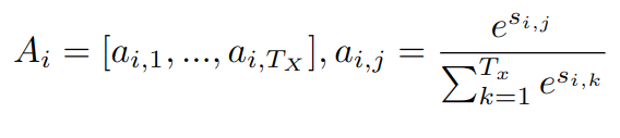
$A_i$ is the vector of attention weights for the i-th output position. It contains $\lvert T_x \rvert$ attention weights, one for each input position. The weights sum to 1 and form a probability distribution over the input, obtained using the softmax function (right). The softmax function is applied to the alignment scores from above.

Using these attention weights, the context vector for the i-th output position is:

\[\large \begin{equation} C_i = H \cdot A_{i} = \sum_{j=1}^{T_x}H_jA_{ij} \end{equation}\]

The context vector $C_i$ for the i-th output position is the dot-product between the attention vector and the hidden states.

Using that context vector, we feed it to the RNN decoder (which is a conditioned language model, as in the original encoder-decoder architecture) and generate a word from it. For each following word, we perform that process again (with different weights, as it will be for different output positions), until generating an “end of sequence” token. To gain more intuition into the attention mechanism, I highly recommend reading Jay Alammar’s post.

Finally, note that the attention weights can be visualized and interpreted as a matrix, where the number of rows is the number of words in the source sentence, and the number of columns is the number of words in the target sentence. Note that each column should sum to 1, and reveal for each word in the translated sequence, what input words affected the translation. Interestingly, observe in the image below the relationships between words in the sentence across languages.

General form

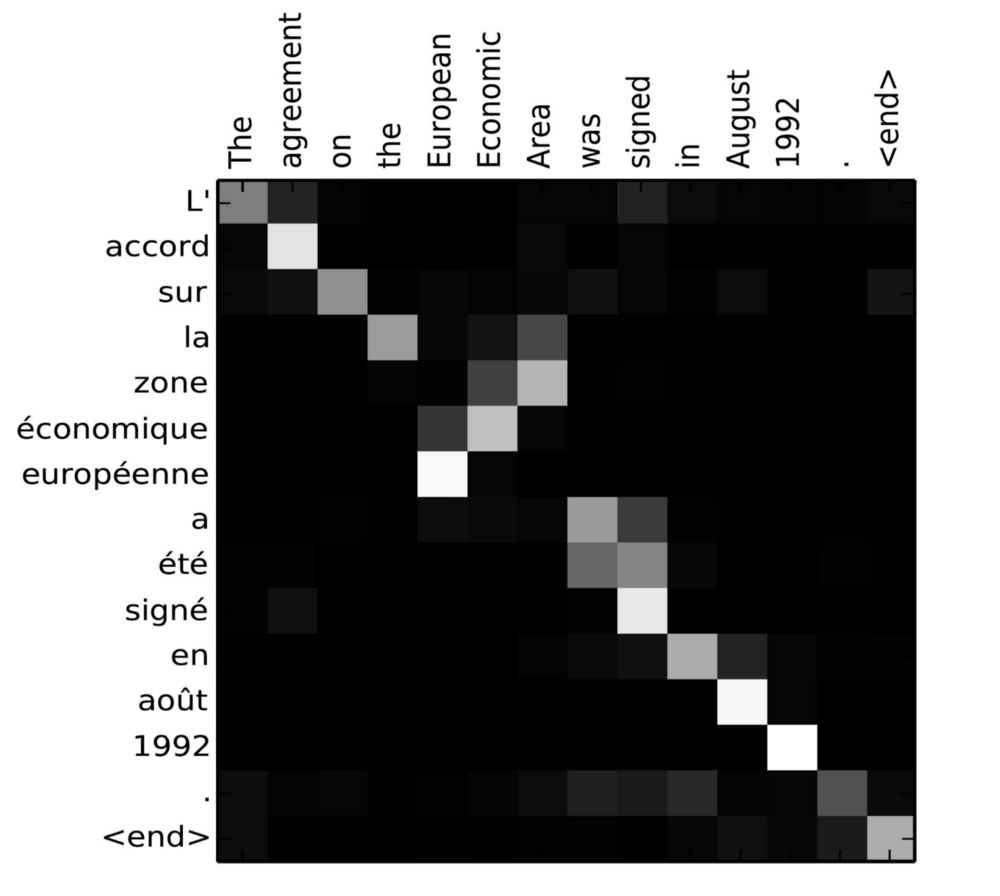
The attention matrix for the sentence “L’accord sur l’Espace économique européen a été signé en août 1992” (French) and its English translation “The agreement on the European Economic Area was signed in August 1992”. Image Source.

Intuition to Attention

Let us quickly recap and change the notation we used to help us continue to the Transformer architecture.

Observe that we basically looked for a way to let the model learn the following: “When translating the i-th word, how it relates to the original sentence j-th word?”. You can motivate this logic intuitively by translating (if you know Hebrew) the sentence: “אני קורא את הבלוג של עומרי” from Hebrew to English: “I read Omri’s blog”. When you translated the 3-rd word (Omri’s), you related both to the last word (עומרי) and to the fifth word (של) to translate the name with a possessive noun.

Let’s be more concise about it. By “relating”, we actually mean taking a weighted average over the input sequence. The weights for the weighted average come from a function that assigns a weight to the positions (input position, output position). Importantly, for every translated i-th word, we want the weights over the input sequence to form a proper probability distribution, so we pass them through the Softmax function.

Generalization of Attention

Now that we have an intuition about the attention mechanism, let us generalize the idea and observe the things needed to construct attention:

A scoring function that operates on two elements and returns an alignment score that signifies how they relate. These alignment scores go through a Softmax function to obtain a probability distribution. Let us denote these elements as Key and Query.
The probability distribution is used to take a weighted average over a third element. This weighted average is the attention. This third element is denoted, simply, as Value.

The intuition behind this naming convention is simple when you keep in mind the translation task. For a given input position (Key), and its corresponding hidden vector (Value), the attention weights tell how it affects the output position (Query). Using this notation, the general attention mechanism can be formalized as:

\[\large\begin{equation} Attention(Q, K, V) = Softmax(Score(Q,K)) \cdot V \end{equation}\]

The general attention mechanism. So far, K and V were the hidden values of the input, Q was the hidden values of the output, and the Score function was the feed-forward network used by Bahdanau et al., 2015.

General form

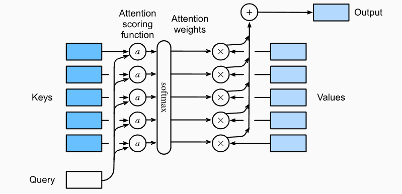
An illustration of the general attention mechanism. Image source.

Attention is Nice - but RNN still has limitations

Encoder-Decoder architectures with attention became highly popular after their introduction in 2015. However, they still rely on RNNs and therefore suffer from a lack of parallelism. Recall that the RNN treats the translation task as a sequential prediction problem. While it is rather intuitive to think of it that way, the sequential nature prevents us to parallelize the training, in contrast to “regular” feed-forward neural network training where all samples can be computed in parallel. This problem becomes critical at longer sequence lengths. Furthermore, although RNN architectures such as LSTM and GRU made longer sequences more tractable, they still don’t perform well for sequences with >100–200 words empirically.

Transformer

Due to the limitations of RNN, one might wonder if it is really needed. A potential suggestion would be to handle the entire input all at once. Instead of feeding the network a single word at every timestep, and letting the network store some kind of memory, just feed the entire sequence at once.

Wait, what? Is it as simple as feeding everything to a single large feed-forward network? Unfortunately, no. The first successful work that removed the use of RNN for sequential problems was the famous Transformer by Vaswani et al., 2017.

General form

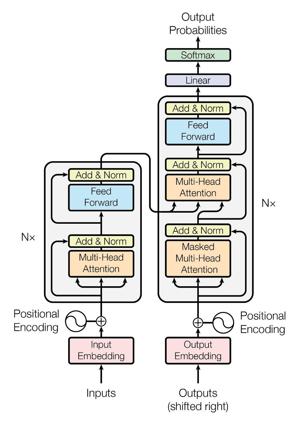
The Transformer architecture. Image source.

A lot has been written on Transformers before, so I will focus only on two parts - self-attention and positional embedding.

Self-attention

Without the ability to learn complicated relationships among the input, our feed-forward network will have a hard time translating sentences or modeling a language. Among others, this is the main reason RNN was so successful - the architecture made it simple to learn relationships between words in the sequence. Specifically, it was easier for the network to learn short-term relationships, as there were direct communication windows between consequence timesteps. By communication window, I roughly refer to a way for the network to pass information between timesteps. Observe that for a sequence of length N, the RNN architecture had a communication window of size N, and as N grew large it was harder for the network to successfully communicate.

How can we give the network a prior to learning complex relationships among the sequence? Luckily, using the general form of attention shown above, we can use the attention mechanism to learn how words in the sequence relate to other words in that sequence. That is called Self-Attention. The only thing we need to specify is how to define the Key (K), Query (Q), and Value (V) matrices given the input sequence. The original paper suggests learning three different matrices that linearly transform the input sequences to K, Q, and V.

General form

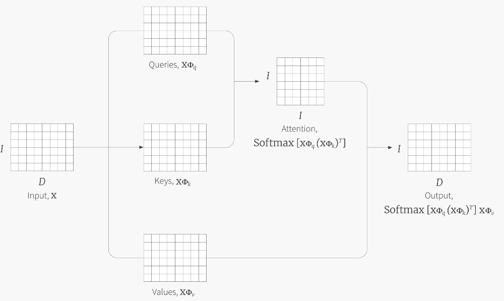
Given an input matrix X, it is linearly projected by three different matrices to the same embedding dimension. Using this Q, K, and V, the attention mechanism is performed. Image source.

Implementation note - Vaswani et al., 2017 used a different scoring function for (Key, Query) pairs. They used the Scaled Dot-Product scoring function:
$$ \large \begin{equation} Attention(Q, K, V) = Softmax(\frac{QK^T}{\sqrt{d_k}}) \cdot V \end{equation}$$

If We Ditched RNN, How Does The Model Know About The Order of Things?

So far we haven’t done anything explicitly to let the network know that it deals with sequential data. We simply feed everything to some fancy architecture of a feed-forward network and hope it to work. Unfortunately, something is missing. We need to explicitly signal the network about the different positions of words in the sequence. To intuitively understand why we need to encode the position of the word in the sentence - simply observe that all words go through an embedding layer, thus producing a vector that represents the word. However, the same vector represents that word regardless of its position in the input. It is clear that we want to give the model different embeddings for the same word in different positions in the sequence, thus we need to somehow encode that position.

A Formal Reason for Positional Encoding

You might have figured out that the above intuition might not be enough. The position of the input is indeed given simply by the fact that the first word is encoded at the beginning of the input vector, and the last word at the end. Why isn’t that enough? This section aims to explain it but feel free to skip over it as it is not crucial to understand and gets a bit mathy. First, we need to consider what happens to the self-attention layer shown above, under some permutation (P) of the input sequence (i.e., swapping words in the input sentence):

\[Attention(PQ, PK, PV) = Softmax(\frac{PQ(PK)^T}{\sqrt{d_k}})\cdot PV = Softmax(\frac{PQK^TP^T}{\sqrt{d_k}})\cdot PV\]

The Self-Attention performed over Q, K, and V after permutation P. Recall that Q, K, and V are a linear transformation of X, therefore applying a permutation P on X results in the above-used PQ, PK, and PV.

Note that when we use the softmax function, we compute the softmax on the dimension of the rows (i.e., normalizing the rows to be a probability distribution). Therefore, since the computation of each row is only affected by the row values, it doesn’t matter when the permutation of the rows is made. Extracting the permutations out of the softmax, we get:

\[\large P Softmax(\frac{QK^T}{\sqrt{d_k}})\cdot P^TPV = P Softmax(\frac{QK^T}{\sqrt{d_k}})\cdot V\]

That means that applying the permutation on the input is equal to the permutation of the output, which is called positional equivariant. Since self-attention is positional equivariant, it means that the same alignment scores will be computed regardless of the order of the words in the sentence. That’s exactly what we see inside the Softmax for the permuted X. That’s obviously not ideal, as we want different alignment scores for different permutations of the input. Therefore, we need to somehow encode the position of the word in the sentence.

Positional Encoding

A naive suggestion for encoding the position would be simply to add a number to the word embedding that specifies the index of the word in the input sequence. However, giving integer indices to the model is problematic for (at least) two reasons. First, it will be hard for the model to generalize to sequences with a different length than the sequences that were given in training. Second, it is a bad practice to give unnormalized integers as input to neural networks.

The next suggestion might be to encode the integer indices by binary vectors. For example, the fifth word will be encoded by the binary number 100 (counting from zero). While it is a better solution than before, feeding such discrete vectors to a network is not a great idea.

Observe that the LSB bit of the integer indices (recall that, in little-endian, the LSB is the rightmost bit, and the MSB is the leftmost bit) changes between each consecutive index (0,1,2,3,4 -> 000, 001, 010, 011, 100 observe how the LSB changes frequently), and the MSB bit changes rarely. Intuitively, you can think of these bits as representing different frequencies (the LSB bit has a high frequency, and the MSB bit has a low frequency). Please read here for more on this intuition. How can we use this intuition to make the binary vectors into continuous representations of the input position?

The solution proposed in the original Transformer paper is to use trig functions (sin and cos) to encode the position. They proposed the following positional encoding:

General form

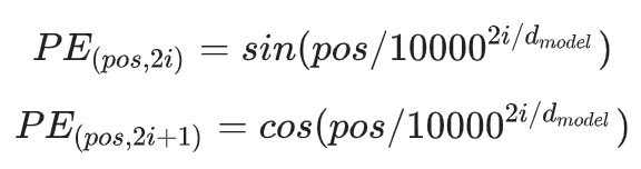
The input position and dimension index denoted with pos and i, respectively. $d_model$ is the positional embedding size.

That might be obscure - why use trig functions? How do they help us encode the position?

To explain that, let’s observe some plots and understand why the trig functions are useful. The code for these plots can be found on my GitHub page. Note that this positional encoding gives a matrix that maps each input position to an embedding vector. In my code, I created this matrix for a sequence with a maximal size of 128 and an embedding dimension of 300. To gain intuition to this positional encoding, let us visualize the embedding vector for the 10-th and the 250-th dimensions:

General form

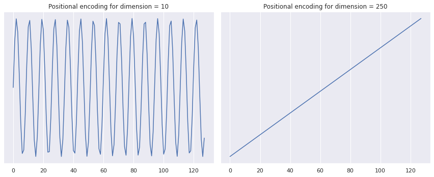
The positional encoding for the 10-th (left) and 250-th (right) dimensions along the input sequence (maximum sequence length is 128).

These plots demonstrate that different positional encoding dimensions describe different relations across input positions. The later dimensions (i.e., the 250th, see right image) gives a monotonically increasing value per input position. That encodes the relation that closer words have more similar encoding than far-away words. However, the first dimensions (i.e., the 10th, see left image) describe a more complicated relation - words that are about ~10 words apart get a similar encoding.

Using this positional encoding allows the transformer access to information about input positions, thus making it a replacement for RNN.

Conclusion

We learned about machine translation, attention, and the generalization of attention. Then, we said goodbye to the RNN architecture and introduced the famous Transformer. We focused on two important building blocks of the Transformer - self-attention and positional encoding. In Part 3, we will highlight several known modern Large Langauge Models (LLM). Then, we will discuss exciting modern work on Transformers and end our journey by understanding CodeX code auto-completion.