From A* to MARL (Part 5- Multi-Agent Reinforcement Learning)
An intuitive high-level overview of the connection between AI planning theory to current Reinforcement Learning research for multi-agent systems. This part (finally!) focus on reinforcement learning (RL) and multi-agent RL.
- A* to MARL Series Introduction
- Single-Agent Reinforcement Learning
- Generalizing to Multi-Agent Reinforcement Learning (MARL)
- Implicit Assumptions
- Conclusion
- Acknowledgment
A* to MARL Series Introduction
Research of Reinforcement Learning (RL) and Multi-Agent RL (MARL) algorithms has advanced rapidly during the last decade. One might suggest it is due to the rise of deep learning and the use of its architectures for RL tasks. While it is true at some level, the foundations of RL, which can be thought of as a planning problem formulated as a learning system, lie in AI planning theory (which has been in development for over 50 years). However, the connection between RL and planning theory might seem vague, as the former is related to deep learning for most practitioners nowadays.
This series of articles aims to start from the classical path-finding problem, with strict assumptions about the world we are tackling (deterministic, centralized, single-agent, etc.) and gradually drop assumptions until we end up with the MARL problem. In the process, we will see several algorithms suited for different assumptions. Yet, an assumption we will always make is that the agents are cooperative. In other words, they act together to achieve a common goal.
It is important to note that this series will focus on the “multi-agent systems path” from A* to MARL. This will be done by formulating the problems we want to solve and the assumptions we make about the world we operate in. It certainly won’t be an in-depth review of all algorithms and their improvement on each topic.
Specifically, I will review optimal multi-agent pathfinding (Part 1), classical planning (Part 2), planning under uncertainty (Part 3), and planning with partial observability (Part 4). Then, I will conclude our journey at RL and its generalization to multi-agent systems (Part 5). I will pick representative algorithms and ideas and will refer the reader to an in-depth review when needed.
Single-Agent Reinforcement Learning
The previous chapters have focused on the question of how to find a plan that achieves a goal under various conditions. All planning frameworks we observed, from MAPF to DEC-POMDP, shared a common assumption - they assume they are familiar with the dynamics of the world in which they operate. We formalized the knowledge they assume about the world through several functions, such as the transition and observation functions. It is time to ask what one should do when facing a planning problem without knowing those functions that model the world?
Intuition for RL
Intuitively, think about yourself, as you wander through life. You certainly do not possess a model of the world in which you operate, and one would further suggest that your reward function is not well-defined. However, let’s assume you have a gut feeling for what makes you happy, and what doesn’t. Moreover, with it, you (kind of) know what will make your future self happy. For simplicity, let’s treat your guts feeling as a reward function that helps you assess different routes in life. To decide what profession suits you, who you should marry with, or even what kind of food you should eat in your mornings, you must experience things, listen to your gut and take actions accordingly. However, even after experiencing and deciding what makes you happy, things might change. You might change due to your new lifestyle, and your gut feeling might change. Things that make you feel good now will not always make you feel good. In a sense, it is not only that you do not own the model of the world, but this model and your gut feeling are also changing, and you need to continuously adapt to it. Making things even more complicated (and real), you might ask how should you decide that you experienced enough and that no other things exist out there that can make you feel even happier?
This model is obviously too simple to describe how a human operates, but it gives intuition to the fashion in which RL problems are modeled, and what challenges they face. The RL agent, much as you do, learns by trial-and-error interaction with its dynamic environment. How much experience does he needs to collect and how well he adapts to new information, is among the critical challenges research in the field is tracking today.
RL is HUGE
Reinforcement learning is a large topic with rapid advancements. For example, a famous book called “Reinforcement Learning: An Introduction” takes more than 500 pages for its introduction. Therefore, this will be far less than even a slight overview of the field. However, I will try to give a high-level intuition for the methods used to solve single-agent RL problems, relying on the intuitions and knowledge you collected from the previous chapters on AI planning.
An RL agent, in our model-free problem, basically only receives rewards from the environment by applying actions. The objective is much the same as was previously. We look for a policy that maps states (or observation of states) to actions such that it would maximize the expected reward. There are mainly two types of methods that search for that policy - value-based and policy-based methods.
Model-based vs model-free RL - A short note
Loosely speaking, model-based RL aims to learn a world model from our experience and then derive a policy from it (using the algorithms for MDPs we learned). Model-free RL aims to directly learn a policy from the experience. The question of “what kind of RL is better”, if any, is being addressed for more than 25 years now. As I personally know more about model-free RL, this is what this post will cover towards MARL.
Value-based methods for model-free RL
One might ask how to use the value iteration algorithm we used to find policies for MDPs. Recall that this algorithm aims to find the value function that corresponds to the optimal policy. With that value function in hand, the optimal policy is to simply pick the action that maximizes the value function for each state. However, as we no longer assume we have access to the transition function, we can not evaluate the value function since it requires computing the mean value function of all possible next states, weighted by their probability. Therefore, we look for a function that we can evaluate only based on experience, that would serve us to find the optimal policy.
Luckily, in 1989, Watkins introduced the Q-learning algorithm. He suggests assigning a value for (state, action) pairs and not states alone. The function that maps a (state, action) pair to a value is called the Q function. It is clear that with the Q function we can still easily find a policy that simply picks the action that maximizes the Q value at each state. So, instead of searching for the optimal policy’s value function, we search for the optimal policy’s Q function. This can be done from the experience we get from applying actions in the world and collecting rewards. So, given some estimation of the Q-value of each state, the update rule of Q-learning is:
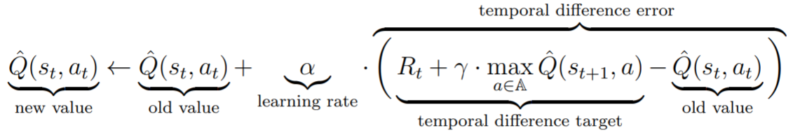
Q-learning update rule.
It basically means that at each step, we take the greedy action according to our currently available Q-function, and update our estimation of the Q-function accordingly. The main part is the temporal difference error. It measures the difference between the current Q-value we had for the current (state, action) pair to the highest Q-value of the next state with the current reward added to it. At convergence, the “temporal difference target” and “old value” parts of the equation should be equal for all (state, action) pairs, and the Q-learning function would converge.
Yet, one might point out that previously we used the value function since it provided optimality guarantees. Does Q-learning provide those guarantees also? Fortunately, it will converge to the optimal policy, when all state-action pairs are visited infinitely often.
However, what “visited infinitely often” means in practice, and how fast can we approach that convergence? How efficient the Q-learning algorithm is in terms of the number of state-action pairs it needs to collect before converging lies in managing the exploration-exploitation tradeoff. This trade-off arises when we need to choose between exploiting our current knowledge (maximizing rewards according to our best currently known policy) and exploring new knowledge and better policies. Simply think of the last time you went to go eat outside. You could choose to eat in one of your favorite restaurants or trying a new one. On the one hand, Choosing the same favorite restaurant every time would certainly provide you with good meals, but you will not find new and even better ones that are out there. On the other hand, if you will constantly try new ones, you will probably experience a large number of bad meals, which you would like to avoid. Read Jin et al., 2019 work for more information on the sample efficiency of Q-learning.
Note that in practice, more often than not, the state and action spaces are too large for the Q-learning algorithm to converge. Therefore, modern approaches for RL utilize function approximators, such as neural networks, to approximate the Q function. A famous example from recent years that combines deep learning with q-learning is the Deep Q-Network.
Policy-based methods for model-free RL
The main idea in Q-learning, and value-based methods in general, is learning the optimal value function and then obtain a greedy policy by picking the action that maximizes it at every state. Another direction to solve RL is to directly learn a policy that determines the probability of choosing an action for a given state. The basic idea is to start with some policy, sample an episode from it, and update the policy according to how well the episode was. The tricky thing is how to determine how to update the policy according to the sampled episode. Policy gradient methods tackle this problem by representing the policy as a neural network and using gradient-based optimization to improve it. The network would aim to minimize a loss function that is the expected reward of a given policy.
Yet, simply saying “gradient-based” does not indicates how we actually derive this gradient? How can we compute the gradient of the expected reward of a given policy? Naively, it would require us to know the state distribution function, which we do not know in RL (as we do not possess the world model). Luckily, a simple formula, named policy gradient theorem, describes the policy’s gradient without knowing the state distribution.
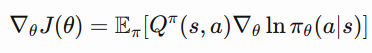
The policy gradient theorem defines the gradient of a policy parameterized by theta.
This formula describes the gradient of a policy, parameterized by theta. The gradient of doing some action a in state s is the expectation of the Q-value of (s,a) times the log-probability of choosing a at state s. Follow the links I note in the next paragraph for details on how to derive this formula.
An issue that policy gradient methods must address is how to estimate the Q-function value. Simple policy gradient methods, such as REINFORCE, use the accumulated future return. Essentially, REINFORCE plays a trajectory from the current policy and uses the information about future rewards at each state to compute the gradient. More sophisticated methods provide better estimates of the gradient, which are both unbiased and with low variance. An example is Actor-Critic methods, which essentially train 2 neural networks. One is the policy network that selects an action for a given state, and the other is a critic network that assesses the value of the state. For a more detailed explanation of policy gradient methods, I refer you to read those great blog posts: 1, 2. Also, OpenAI’s tutorial and code of Policy Gradients are highly recommended.
Between policy-based and value-based
While the two approaches described above might not seem compatible, there exist algorithms that try to involve both of them. A famous example is the DDPG method that learns both a value function and a policy using gradient descent. One might note that Actor-Critic methods, which are mentioned before, are also a mix of both approaches. While it is true, a critical advantage of value-based methods is that they are off-policy. It means that it can learn from past experience, which is not even collected by a policy the agent possesses. However, Actor-Critic is an on-policy method, and it means that it can only learn from episodes generated by the policy it possesses (otherwise, we will perform steps based on gradients of another function). On the other hand, the DDPG algorithm (usually used variant, at least) is an off-policy method. Moreover, it tackles continuous action spaces, which is a problem for value-based methods. A critical idea behind DDPG is to learn a deterministic policy. While it is not intuitive at first glance how can we compute the gradient for a deterministic policy, in 2014 David Silver revealed it to be as straightforward as in the original policy gradient method. Check OpenAI’s tutorial on DDPG for more details on it.
Quick Recap
Before examining the multi-agent case of RL, let’s do a quick recap. We introduced RL as the framework to solve planning problems by directly interacting with an environment in which we do not possess a world model. Specifically, we focused on the model-free path, where we wish to directly learn how to act, without deriving the world model. We learned about the two main approaches for tackling RL problems - value-based and policy gradients methods. The first approach aims to derive a policy based on its approximation of the value function for each (state, action) pair. The second approach aims to directly optimize a policy based on the interaction with the environment. Common to those approaches is the utilization of neural networks as function approximations to efficiently solve RL problems.
Generalizing to Multi-Agent Reinforcement Learning (MARL)
As we have seen along our path, naive approaches convert the multi-agent problem to a single meta-agent problem and decide for all the agents using a centralized controller. However, in those approaches, the number of actions typically exponentially increases, which makes the problem intractable, just as we saw for MDPs and POMDPs. Furthermore, if we assume that the agents are distributed but all agents know about all other agents, they still need to solve the coordination problem, which we observed both for MMDP and MPOMDP. Specifically, since multiple optimal policies may exist, they need to learn to coordinate which joint optimal policy to follow. Both of those scenarios, of a single meta-agent and fully observable agents, are out of scope for today. However, the ideas of MARL for those scenarios resemble the ideas we have seen in previous chapters.
Value-based methods for MARL
Before diving into specific value-based MARL algorithms, we need to revisit one critical component of Q-learning - experience replay. It is a fixed-size buffer that holds the most recent transitions collected by the policy. As greatly described in the seminal work of Lin: “By experience replay, the learning agent simply remembers its past experiences and repeatedly presents the experiences to its learning algorithm as if the agent experienced again and again what it had experienced before. The result of doing this is that the process of credit/blame propagation is sped up and therefore the networks usually converge more quickly. However, it is important to note that a condition for experience replay to be useful is that the laws that govern the environment of the learning agent should not change over time (or at least not change rapidly), simply because if the laws have changed, past experiences may become irrelevant or even harmful.”
This quote from 1992 is still highly relevant today. Experience replay is a critical component of modern variants of deep Q-learning. Moreover, in 2020 a research by Fedus et. al. that analyzed the effect of different aspects of experience replay, such as the number of past experiences we store and how many times we “play” those past experiences revealed how critical a good setup of the experience replay mechanism is for modern Q-learning based RL methods to converge.
However, when generalizing RL to the multi-agent scenario, a problem occurs. At MARL, each agent is faced with a moving-target learning problem: the best policy changes as the other agents’ policies change. This is also called nonstationarity, and its cause is that the actions performed by other agents might affect the state of the environment. But, if the environmental laws change in time, it is not clear how can we use past experience. And without experience replay, the Q-learning-based approaches can be hard to train due to the sample inefficiency and correlation among the samples. Does it remind you of the problem we faced with DEC-POMDPs in the last chapter? Indeed, we faced a similar problem where we could not plan for each agent in the DEC-POMDP scenario since the Markov property was not satisfied by using only each agent’s observations.
Therefore, the naive idea of simply decentralizing the RL agents, with each one learns only by its observations of the environment should not be a good solution. This algorithm is called Independent Q-Learning (IQL), and while it works for small problems, for large problems that require deep learning, convergence is highly challenging. And here comes another idea we already saw before - instead of searching for the optimal joint policy, let’s try to search for a nash equilibrium joint policy. Recall that nash equilibrium means that the policy assigned for each agent is the best response strategy for the policies of all other agents. This idea was used by Fuji et. al, 2018, and highly resembles the idea of JESP for DEC-POMDPs back in 2003 that we introduced in the last chapter. They suggest training only one of the agents at each time while keeping all other agent’s policies fixed.
While IQL is appealing as it avoids the scalability problems of the multi-agent system, it does not scale to large problems that are solved with deep learning-based methods, as they heavily rely on the experience replay mechanism. Therefore Forester et. al, 2018 proposed two algorithms to enable the use of experience replay in IQL-based algorithms for MARL. The first algorithm basically tries to decay obsolete data from the experience replay by assigning a lower probability to sample it. The second algorithm proposes to augment the past experience with some metadata (called a fingerprint) that disambiguates the age of the data sampled from the experience replay. Both algorithms successfully combine experience replay with Deep IQL, and their experiments suggest the fingerprint-based solution achieves superior results.
Policy-gradient methods for MARL
In multi-agent RL, the noise and variance of the rewards increase which results in the instability of the training. The reason is that the reward of one agent depends on the actions of other agents, and the conditioned reward on the action of a single agent can exhibit much more noise and variability than a single agent’s reward. Therefore, training a policy gradient algorithm would not be effective in general.
One successful implementation of policy gradients and value-based methods is MADDPG, which extends the DDPG algorithm to the multi-agent case. It relies on an idea we have seen in DEC-MDP and DEC-POMDP, where training (planning, for MDPs) is centralized, but the execution is decentralized. Thus, the policies may use extra information to ease training, but this information is not used at execution.
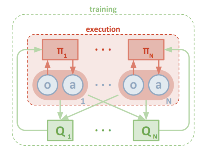
MADDPG high-level architecture. Each agent trains a DDPG algorithm, where the critics can access all actions and observations during training, but only the single agents’ actions and observations at execution.
Each agent in MADDPG trains a DDPG algorithm, which means training two networks - a policy and a critic. At training, all critics have access to information from other agents (their policies, actions, and observations). The motivation for it is that during training, the environment becomes stationary for the critics, as they know all other agents’ policies and actions. Since the critic is not used at execution, we can discard it and simply use the agent’s policy network in a decentralized way.
While MADDPG made significant improvements, it has one crucial limitation. The input size of the critics grows linearly with the number of agents. Therefore, it does not suit environments with a large number of agents.
MARL in the broader sense
As you might have guessed, we only focused on a specific problem of MARL, which deals with planning for cooperative agents with shared rewards. Yet, in the broader sense of multi-agent learning, one might ask many other interesting questions, such as how non-cooperative agents learn, how people learn in the context of other learners and how can agents learn without an explicitly defined reward function. I refer you to the great paper “If multi-agent learning is the answer, what is the question?” for more information.
For a modern survey of cooperative MARL, I highly recommend this survey, which covers what we have seen in this post and many other methods that solve cooperative MARL.
Implicit Assumptions
As this series concentrated on dropping assumptions, I feel it is desired to remind you that we are constantly making implicit assumptions, and noting them is a crucial skill that all of us should practice. Let’s try to identify some more assumptions we made throughout this series. We assumed all actions to have the same duration. Also, we assumed that all agents are synchronized on this duration. Furthermore, we assumed some definition of a goal, or a reward function, while we clearly do not possess one in our life. And even if we possess a goal/reward definition, we assumed that we plan for rational agents that wish to maximize its expectancy. What other interesting assumptions do you find? Also, have you noticed the assumption of “identifying implicit assumptions is something we can practice”?
Conclusion
Well, this was a long journey. We started it way back in the origins of the pathfinding problem. When we extended it to MAPF (Multi-Agent Path Finding), we immediately saw that generalizing a single-agent problem to multi-agent is not trivial. Then, we went through a richer framework for planning problems, namely STRIPS/PDDL languages. We kept trying to generalize to the multi-agent case and saw some recurring patterns, as the aim to find decoupled agents and exploit this independence between them to more efficiently find a plan.
Following, we acknowledged that most systems entail some level of uncertainty, and we first added control uncertainty and then added sensor uncertainty. Those uncertainties made us look for policies that map actions to states, rather than a fixed plan. We formalized those uncertainties in MDPs and POMDPs, which are the most common framework for AI planning today. Then, we generalized those frameworks for the multi-agent case and again observed recurring issues. For example, the coordination problem, the formulation of the “centralized planning, decentralized execution” line of solutions, and the violation of the Markov property induced by the multi-agent case.
Finally, we asked how can we plan when we do not possess a model of the world. This is where we entered the land of (model-free) RL. We saw that the methods we used to solve MDPs can be generalized for RL (Q-learning). Also, we saw that basically the same issues we tackled at generalizing MDPs and POMDPs are still relevant at MARL and the ideas behind the solutions from planning might serve us to solve MARL.
I learned a lot by writing this series. Hope you learned some too. Feel free to contact me with any questions/suggestions/corrections.
Acknowledgment
I want to thank Roni Stern, my MSc thesis supervisor. My interest in this area and large parts of this blog series stems from the wonderful course he teaches on multi-agent systems at Ben-Gurion University, which I had the privilege to take.