Deep Learning Optimization Theory - Introduction
Understanding the thoery of optimization in deep learning is crucial to enable progress. This post provides an introduction to it.
Introduction
Over the last decade, deep learning flourished in both academia and industry. Both real-world and academic problems that were notoriously hard for decades, such as computer vision, natural language processing, and game-playing, are now being solved with high success using deep learning methods.
However, despite those significant improvements in deep learning, the theoretical understanding of its success lags behind. Our understanding ranges from conventional wisdom and intuitions that are based on experiments to deeper analysis of toy problems that do not resemble the true complexity of real-world deep learning architectures. This blog post aims to highlight interesting lessons learned from deep learning theory research that challenged conventional wisdom.
In general, deep learning consists of the following three pillars:
- Expressivity - What functions can we express with a neural network? How efficient is one neural network concerning the other in terms of the set of functions they can represent? What inductive biasesexist in modern neural networks?
- Optimization - How can we find the best weights for our neural network for a given task? Can we guarantee to find the best one? How fast can we do it?
- Generalization - Why does a solution on a training set generalize well to an unseen test set? Can we bound the generalization error?
This post will focus on optimization. The reader is assumed to be familiar with SGD, deep learning, and some background in optimization.
Deep Learning Theory- Optimization
Optimization of convex functions is considered a mature field in mathematics. Accordingly, one can use well-established tools and theories to answer the questions described in the last paragraph for optimization. However, optimization of complicated non-convex functions is hard to analyze. Since the optimization of deep neural networks (yes, linear ones also) is non-convex, how can we attempt to answer those questions? One might seek wide empirical evidence that SGD converges to global minima on real-world problems. The other might look for a rigorous theoretical explanation of its convergence and the conditions for it to occur. As both of those approaches, the experimental, and theoretical help push our knowledge further, in this blog post I will present representative works from both approaches. The first approach I will represent is the experimental approach.
An Experimental Approach
The work “Qualitatively characterizing neural network optimization problems” by Goodfellow et. al., suggested a simple tool to tackle the above-mentioned optimization questions for specific practical networks and problems. Let’s assume you trained your network to convergence for a global optimum (training loss near zero). Now, take the weights at initialization and the weights at convergence, and simply evaluate your loss function at a series of points on a line in parameter space between your initial weights and convergence weights. More formally:

Sampled thetas along the line between \(\theta_i\) (weights at initialization) to \(\theta_c\) (weights at convergence).
As we suspect the loss function to be highly non-convex, it would be hard to imagine the behavior of the loss function along this line. Surprisingly, performing this experiment on a feed-forward neural network trained on MNIST reveals the following behavior:
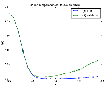
A linear interpolation experiment on a fully connected network with ReLU activations, trained on MNIST dataset. This shows that the objective function is smooth within the line between the initial and target parameters of the model.
Un-intuitively, we observe that the loss function across this line is a continuous monotonic decreasing function. This suggests that while the loss function itself is highly non-convex, there is an “almost convex” path to the convergence point. Moreover, other experiments with other architectures (CNN/RNN) revealed a similar phenomenon. Please read the paper for more details. If you are interested in experimenting with it yourself, you can use my implementation for it.
Now that we know that a smooth monotonically decreasing path from initial weights to convergence exists, one might ask - does SGD follows this linear path? To answer this question, we are looking for a way to assess “how SGD progressed along the line if projected on it”. Also, in case that those weights are not on that 1D subspace, we would like to assess “how far are they from the line”. We denote the distance along the line by α and the distance from that line by β. Before diving into the specifics of how α and β are mathematically defined, observe the following:
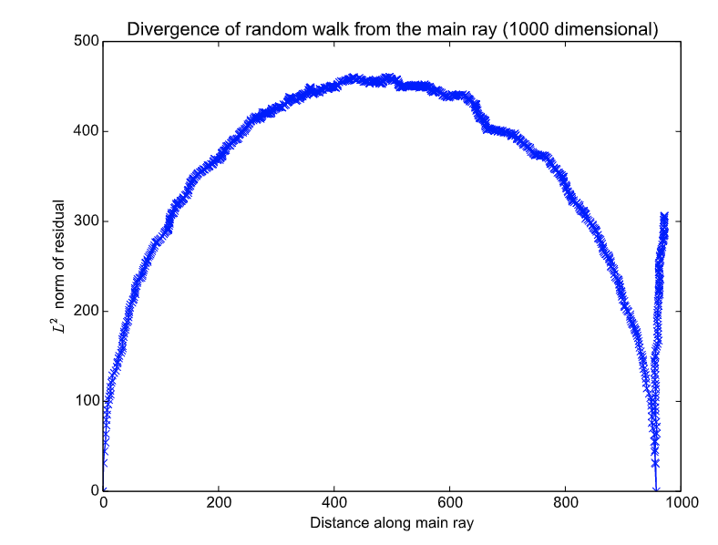
Horizontal axis - α (progress along the linear path - 0 is at init, 900 is at final model). Vertical axis - β (distance of SGD weights at time T from the linear path).
Interestingly, it seems like as SGD progresses, it has a symmetric pattern of diverging and converging to the line. At first, it diverges from it and, at almost complete symmetry, converges back to it.
Let’s quickly describe the mathematics of those parameters. If you only care for intuition, skip the following paragraph, or just refer to my implementation if you would like to run this experiment yourself.
Let us define u as the unit vector pointing from \(\theta_i\) to \(\theta_c\). We can describe the linear path between \(\theta_i\) to \(\theta_c\) as: \(\theta_i\) + \(\alpha(t)*u\), where \(\alpha(t)\) is a scalar representing “how much progress has been made on-the-line”, defined as:

For a timestep t, compute the progress done by SGD projected on the line from initialization to convergence.
Now we have \(\alpha\) that specifies the magnitude we progressed along the line. The missing component is the distance from it. Let us define another unit vector v that is pointing in the direction from \(\theta_t\) to projected progress on the line.

For a timestamp t, β is the norm (distance) of the weights of SGD from the projected progress of them on the line from initialization to convergence.
And that’s all needed to reproduce the experiment shown above!
Revision for Modern Neural Networks
Looking back on those results from 2014 today, after immense progress in the field of deep learning, one might ask to revisit the phenomena observed in the original paper. Indeed, Jonathan Frankle at 2020 experimented with modern NN architectures and datasets and found that the situation might not be as nice as it was with simple architectures on simple datasets.
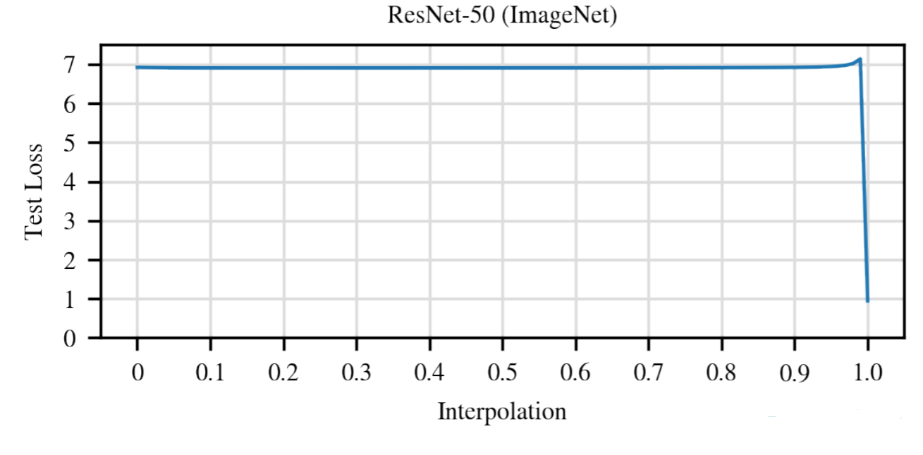
The linear interpolation experiment was revisited with ResNet-50 on the ImageNet dataset. Loss is no longer monotonically decreasing from init to convergence.
Surprisingly, in modern NN architectures, he did not find this phenomenon to occur. More strangely, he found that this experiment with ResNet-50 on ImageNet resulted in the peculiar observation shown above. Along the line between initial weights to convergence, the loss stays with almost the same value, then increases by a small amount and drops to convergence.
A Possible Explanation (Opinionated)
The work “Visualizing the Loss Landscape of Neural Nets” by Hao Li et. al. provides a method to visualize loss functions curvature. Using their visualization method (which I will do in future posts!) they explore how different network architectures affects the loss landscape. Surprisingly, adding skip-connections to a deep neural network reduces remarkably the landscape from a chaotic to be “almost convex”, as shown in the picture below.
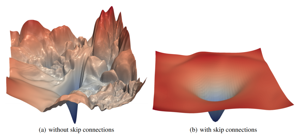
A possible (opinionated) explanation for the phenomena observed with ResNet-50. If we assume the skip connections of ResNet to “convexify” the loss function, it may explain the “non-changing loss until a sudden drop to global minimum” observation. Image source.
This change might bridge the phenomena Goodfellow et. al. found in 2014 and Frankle in 2020. At the right side of the image, it is clear that there is a large flat region of interpolation between initialization weights (assumed to be somewhere on the flat region) to the convergence weights. Moreover, throughout this interpolation, the loss value does not change much.
To conclude the experimental approach, one could say that they gave us a sense of optimism regarding the difficulty of the optimization problem. It suggests that the problems are not as hard as we might have thought. How can we rigorously prove (or disprove) this hypothesis?
A Theoretical Approach
While the experimental approach gives rise to the conventional wisdom that helps us push deep learning to interesting application usages, it does not provide sound explanations for the observations we have, as seen with the revisited experiments on modern architectures in the previous section. Specifically, I will present one approach that aims towards a better understanding of the loss landscape and therefore its optimization characteristics. Another approach is understanding the trajectory of gradient descent itself, which I will cover in future posts.
How Nice is The Loss Landscape?
The work “On the Quality of the Initial Basin in Overspecified Neural Networks” by Itay Safran and Ohad Shamir, approaches the problem by an attempt to model the geometric structure of the (non-convex) loss function. The motivation for this approach is that hopefully, we would find that the loss landscape is convenient for optimization (and even more specifically, local search algorithms such as SGD). The observations we have seen before about the empirically existing monotonic decreasing paths encouraged researchers to explain this phenomenon.
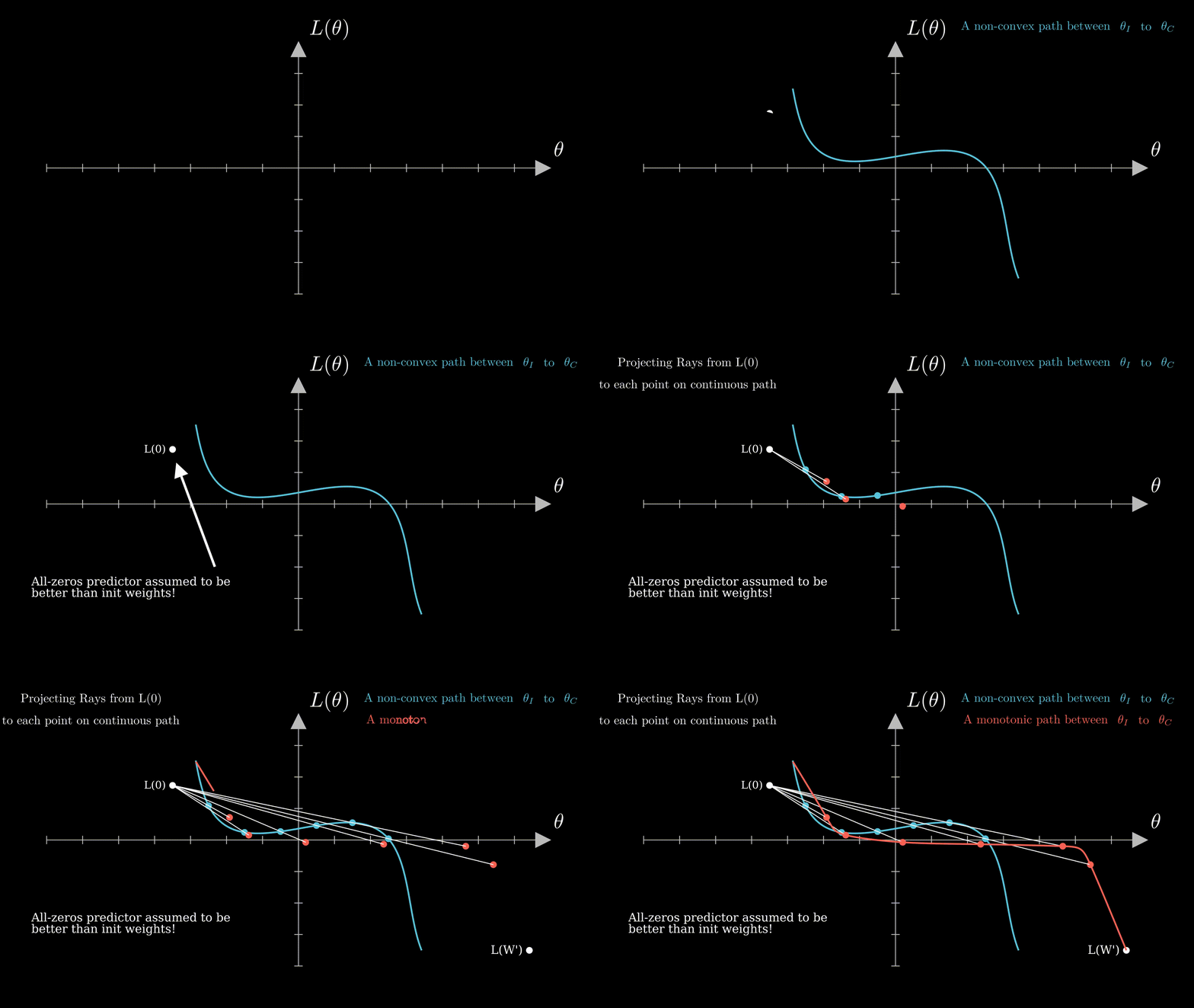
Specifically, this work provides the following theorem: Given a fully connected network, its weights at initialization and convergence, and a convex loss function, there exist a monotonically decreasing path that starts from that initialization point and ends up with the same loss value (as the convergence point). The mainly non-trivial assumption being made to prove that theorem is that the loss of an all-zero predictor is smaller than the loss at initialization.
Even though this assumption is not being held by modern neural networks (due to recent advancements in weight initialization techniques), their result is highly interesting as it lies in line with the empirical results we saw earlier. They prove that under their assumptions, there is an “easy way for optimization”.
While providing the full proof and subtle details of their theorem is certainly out-ot-scope for a blog post, let us try to understand the general idea. The main approach in their proof is to create for each point in the continuous path from init to convergence, create a corresponding point in the monotonically decreasing path. How do they construct the corresponding point? They provide intuition for the special case of the squared loss:

The squared loss, evaluated on a neural network N, parameterized by weights W, for a dataset with m samples.
Since the last layer of the neural network under this objective is linear, note that multiplying the last layer by some scalar c, corresponds to multiplying the networks’ outputs. So, given some weights W(λ) (where 0≤λ≤1 defines the path between init to convergence), we can multiply the last layer by a scalar c≥0 and receive the corresponding weights (denote by W`), with the objective:

The corresponding objective for W(λ) by multiplying its last layer by a scalar c.
Note that for c=0, this objective is the mean of \(Y^2\). For c=∞, it is ∞ also. It basically says (using the intermediate value theorem) that we can tune c to get any objective value from the mean of \(Y^2\) to ∞. Now all that remains is finding for each W(λ) its corresponding c such that we get the desired monotonically decreasing path!
A Visual Recap
Grasping this idea might be challenging. To make it easier for you, I made (using the great manim tool, originated from 3B1B) a short GIF that illustrates the idea of the proof:
Conclusion
Our first step towards understanding the optimization of deep learning models was overall optimistic. Previous knowledge in optimization teaches us that optimizing high-dimensional non-linear and non-convex problems is a notoriously hard problem. However, experiments on real-world models (FC/CNN/RNN) provided optimistic results. Moreover, theoretical analyses of the loss landscape were optimistic as well. In some sense, both of those approaches (experimental and theoretical) suggested that the problems we solve with SGD in deep learning might be far easier to solve than what one might think. However, jumping to 2020, we observed that revisiting those experiments with modern architectures and datasets revealed different phenomena. While those early findings are encouraging from the practitioner’s point of view, the need for a theory behind the convergence of SGD is still needed. Fortunately, researchers in recent years achieved remarkable results, some of which took different approaches to the landscape approach, which I will review in future posts.
Acknowledgment
I want to thank Nadav Cohen for teaching a great course on the theory of deep learning at Tel-Aviv University.