From A* to MARL (Part 4 - Planning Under Uncertainty & Partial Observability)

An intuitive high-level overview of the connection between AI planning theory to current Reinforcement Learning research for multi-agent systems. This part focus on POMDPs and planning under partial observability.

• A* to MARL Series Introduction
• Single-Agent Planning Under Partial Observability
  • POMDP - Representing Partial Observability
  • Markov Property in POMDP
  • Belief State MDP
  • Finding the Optimal Policy - Solving POMDPs
  • Quick Recap
• Generalizing to Multi-Agent POMDP
  • Multi-Agent POMDP - MPOMDP
  • Decentralized POMDP (DEC-POMDP)
  • Approximate Solutions for DEC-POMDP
• Conclusion
• Acknowledgment

A* to MARL Series Introduction

Research of Reinforcement Learning (RL) and Multi-Agent RL (MARL) algorithms has advanced rapidly during the last decade. One might suggest it is due to the rise of deep learning and the use of its architectures for RL tasks. While it is true at some level, the foundations of RL, which can be thought of as a planning problem formulated as a learning system, lie in AI planning theory (which has been in development for over 50 years). However, the connection between RL and planning theory might seem vague, as the former is related to deep learning for most practitioners nowadays.

This series of articles aims to start from the classical path-finding problem, with strict assumptions about the world we are tackling (deterministic, centralized, single-agent, etc.) and gradually drop assumptions until we end up with the MARL problem. In the process, we will see several algorithms suited for different assumptions. Yet, an assumption we will always make is that the agents are cooperative. In other words, they act together to achieve a common goal.

It is important to note that this series will focus on the “multi-agent systems path” from A* to MARL. This will be done by formulating the problems we want to solve and the assumptions we make about the world we operate in. It certainly won’t be an in-depth review of all algorithms and their improvement on each topic.

Specifically, I will review optimal multi-agent pathfinding (Part 1), classical planning (Part 2), planning under uncertainty (Part 3), and planning with partial observability (Part 4). Then, I will conclude our journey at RL and its generalization to multi-agent systems (Part 5). I will pick representative algorithms and ideas and will refer the reader to an in-depth review when needed.

Single-Agent Planning Under Partial Observability

In the previous post, we learned how to represent a planning problem with uncertainty with the MDP framework. Specifically, the uncertainty we dealt with stemmed from control errors, i.e. we had uncertainty about the outcome of our actions. Now, we will extend our view of uncertainty to include sensor errors or limitations. This kind of uncertainty arises when we are not able to determine what the state of the world exactly is. Furthermore, we might not even know for certain what is the initial state. In such cases, we say that the world is partially observable.

A simple motivating example of sensor errors and limitations is planning for the recycling robot. The recycling robot can pick objects and drop them in different trash cans while obeying some predefined logic of what objects should be placed in which trash cans. Yet, while picking an object, the robot does not know if the trash can is full or not, since his camera is not pointing towards the trash can. This illustrates a sensor limitation. Moreover, when the robot camera does point towards the trash can, it has some inherent error and might not identify that it is full. This illustrates a sensor error. Both of those examples produce a partially observable system.

AlphaBet EveryDay robot, staring (with uncertainty) at trash cans.

POMDP - Representing Partial Observability

To represent this added uncertainty, the Partial Observability MDP (POMDP) has been suggested to extend the MDP by incorporating observations and their probability of occurrence conditional on the state of the environment. Remember that we defined MDP by actions, states, transition function, and reward function. Now we add a set of observations and a corresponding observation function that assigns a probability for each triplet of (s,a,o). It defines the probability of observing o after applying action a at state s. Formally, the observation function is defined as:

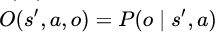
The observation function. It models the probability of observing o when action a is applied in state s’.

Markov Property in POMDP

A critical assumption we made when introducing MDPs was assuming the Markov property holds. Remember it simply means that we assume that the future is independent of the past given the present. Does this property hold for POMDP? Unfortunately, no.

Returning to our recycling robot, we use it to illustrate the violation of the Markov property. Assume the robot already threw several items into some trash can and observed it to be full (with some probability). Now he is picking an item that needs to be thrown into that trash can also. It clearly can not deduce from his current observation (i.e., where the item it aims to recycle is) if the trash can is full. It does know that the trash can is full from its history of actions and observations. However, since the future is now dependent on the past, the Markov property is violated.

A naive solution is extending the definition of current observation to include all actions and observation history. In this case, the Markov property holds, yet we need a policy that maps each possible history to an action, which is highly ineffective. A better solution maintains only the sufficient information it needs to satisfy the Markov property. Going back to our recycling robot, we can intuitively see how ineffective would be to store all information. Let say we threw 100 items into the green trash can and observed it to be full (with some probability). We now observe another item that should be thrown into the green trash can. Instead of remembering all 100 observations we made, we could maintain information that indicates if the trash can is full. However, how do we decide if the trash can is full or not? Since we only have observations (and not a certain state), we assign a probability to it being full. Each time we observe the trash can, we update that probability accordingly. This probability is sometimes called a sufficient statistic. It basically says that maintaining this probability is equivalent to storing the whole history. Therefore, we say that the Markov property holds if the state consists of this maintained probability. We call this state a belief state. The resulting MDP framework that encompasses the partial observability through belief states is called a belief state MDP. Next, we will see how to maintain and update those belief states according to observations, and how to derive a reward for each belief state from the regular reward that is defined on states.

Belief State MDP

So, how do we actually maintain the belief state? Specifically, given a currently assigned probability to each state, an action we perform, and an observation we observe, how do we update those probabilities? Formally, we ask how to compute:

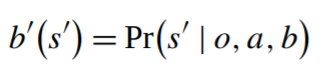
Updating the belief state b’ probability of state s` after being in belief state b, applying action a, and observing o.

Using basic probability theory (Bayes’ rule and marginalization), as described in section 3.3 of this paper, we find that this probability is being updated according to the transition function, observation function, and current belief state. Formally, the formula to update the probability of state s’ is:

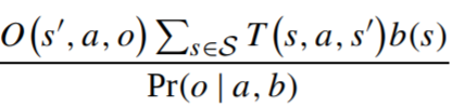
The updated probability of state s’, after applying action a and observing o at belief state b(s). T and O are transition and observation functions.

Given this definition of belief state and the method of updating the belief state according to observations, we change the definition of the transition function accordingly. Remember that it assigns a probability of arriving state s’ after applying action a at state s. We simply replace the regular (certain) state with the new belief state.

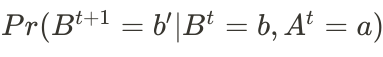
The belief state MDP transition function. It assigns a probability of arriving belief state b’ after applying action a at belief state b.

Finally, we define the reward function as follows:

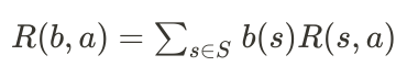
The belief state MDP reward function. It computes a weighted average of the original reward by multiplying it by the probability of each state.

Given this definition of a belief state MDP, which is a representation of the POMDP problem that satisfies the Markov property more efficiently, we now seek algorithms that find the optimal policy for it.

Finding the Optimal Policy - Solving POMDPs

Extending the policy definition from MDP is trivial. For MDP, we search for a policy that maps states to actions. For POMDP (represented as belief state MDP), we search for a policy that maps from beliefs to actions. The optimal policy remains the policy that maximizes the expected rewards.

The main algorithms we looked at previously for finding an optimal policy were Value Iteration and Policy Iteration. Intuitively, those algorithms aim to iteratively improve the policy by comparing its selected actions with a greedy better action. Specifically, we formalized this problem as finding a policy that optimizes the value function. We defined how to evaluate the value function for a given policy at a given state and we defined a method to check if a given policy is optimal. In case of finding a choice of action that improves the value function, we update the policy accordingly and continue until convergence.

However, applying those algorithms to the belief state MDP is not trivial, as they assume a discrete state space, while the belief state is continuous. We need to define an optimization problem that tackles this continuous state. Intuitively, we want to exploit the fact that (generally) the actions chosen by a given policy do not change with “slight changes” to the belief state. Returning to our recycling robot, assume that the optimal policy is to throw an item into the corresponding trash can if the trash can is empty with 90% confidence. Evaluating the value function of this policy naively would require evaluating it over every possible belief state (which is infinitely many times). However, observe that the choice of the action only changes at the tipping point of “90% estimation that the trash can is empty”. Essentially, we look for algorithms that exploit this observation and do not need to evaluate the value function for all belief states. Next, we will define the value function for a belief-state MDP and the basic idea behind those algorithms.

Recall the definition of the value function for MDP as a weighted average of the values of possible next states, weighted by their probability of occurring:

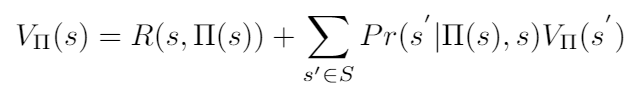
The value function of policy π, evaluated at state s.

Generalizing that value function to include partial observability is done by computing the expected value of the next state. This is the weighted average of the value of the next state weighted by the probability of observing each possible observation.

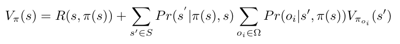
The POMDP value function of policy π, evaluated at state s. Note that the difference is that we take a weighted average of all possible observations.

However, we already know that the agent will never know the exact state of the world, so we need to define the value function for a belief state. We get this by (once again) computing a weighted average of every possible state weighted by its probability of occurring (i.e., the belief state).

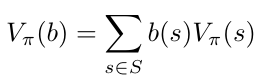
The belief-state MDP value function of policy π, evaluated at belief state b.

Note that we can represent this value function in vector notation as the dot product of two vectors:

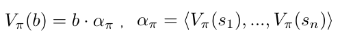
The belief-state MDP value function is represented in vector notation.

Now, we can define the problem of finding the optimal policy for a belief-state MDP as the following optimization problem:

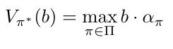
The optimal policy is the policy that maximizes the value function of the belief state MDP.

Observe that this function is piece-wise linear (in b) and convex. If you wonder why this is the case, let look at the following value function for a belief state of a system with 2 possible states. Since it has 2 possible states, the belief state can be represented as one number (as those probabilities sum to 1). Therefore, in the figure below, the x-axis represents the probability we assign for the system to be in state s1 and the y-axis is the value function. Each one of the lines represents a different policy (P1, P2, and P3 accordingly), and it is clear that those policies are linear with respect to the belief state. Furthermore, the bold line, which describes the optimal policy for each belief state, selects the action suggested by the policy that gives the highest value function. This optimal policy is piece-wise linear and convex.

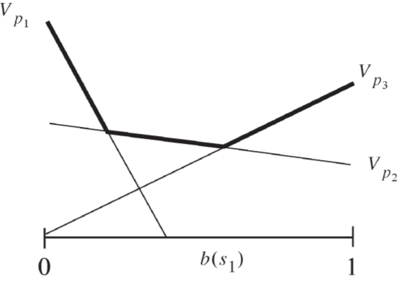
The value function of several policies is evaluated for the belief state of a system with one state only.

Therefore, the problem of finding the optimal policy reduces to finding those bold lines induced by the policies with the highest value for each belief state. This is the basic idea underlying algorithms that find the optimal policy for POMDPs. I will not dive further into how those algorithms actually do it, but I encourage you to read this great paper about POMDPs optimal algorithms.

Quick Recap

The last part was pretty heavy, so let do a quick recap before generalizing to multi-agent POMDPs. We were looking for algorithms that find the optimal policy of the POMDP. However, simply using the previously introduced algorithms is not a great idea, as they assume discrete state space. Yet, we observed (intuitively) that the selected action changes in only several points for a given policy. Therefore, we looked to exploit this observation and search for those points where the optimal policy needs to change its action selection policy. Specifically, we found that the optimal policy value function is piece-wise linear and the problem reduced to finding the set of policies (which were lines in our simple example) that we need to “piece together” to build the optimal policy.

Note that the set of points that the optimal policy need to change its action might be very large (or even continuous) in extreme cases, but we ignore it for simplicity.

Generalizing to Multi-Agent POMDP

Same as we saw with MDPs when generalizing to a multi-agent system it is critical to distinguish between centralized and decentralized systems. If the system is truly centralized at execution, we have a central entity that derives an optimal joint plan. It simply observes all observations and derives the joint action at each joint belief state for all agents. While this centralized system is, in general, simpler to solve, the centralized execution assumption is hard to make. Moreover, this centralized system is essentially a POMDP, so we move on to systems where the execution is decentralized.

Multi-Agent POMDP - MPOMDP

Analogous to what we saw previously when generalizing MDP to decentralized multi-agent systems, we first consider the Multi-agent POMDP (MPOMDP) framework. Basically, it is the generalization of MMDP to a system with partial observability. At MPOMDP, each agent has access to the joint POMDP problem and it solves it optimally. Then, at execution, we need to solve the coordination problem. Remember that the coordination problem arises when there is more than one optimal policy for some agents, and they need to coordinate which policy they chose to act optimally together at execution. We noted several approaches to address this coordination problem. One common for MPOMDPs is by adding each agent the ability to communicate (modeled by an action) its observations to all other agents instantaneously and without a cost. That way, the MPOMDP problem is reduced to simply solve a big POMDP problem. However we choose to solve the coordination problem, the MPOMDP model still makes non-trivial assumptions. First, in most cases, the agents simply can not observe all observations made by all agents. Second, even if they do observe all observations, as we saw in MMDP, solving the full POMDP problem by each agent is intractable for systems with more than a few agents.

Decentralized POMDP (DEC-POMDP)

Therefore, the Decentralized POMDP (DEC-POMDP) framework is suggested. It assumes that individual agents only know about their observations and actions. The first difficulty at this framework concerns the definition of the belief state. For POMDP, we summarized the history in terms of a belief state. It was a crucial step toward utilizing dynamic programming methods, as the belief state satisfies the Markov property without maintaining a full history of actions and observations. In essence, given the belief state, we could optimally plan for the future. However, at DEC-POMDPs, summarizing the individual agent’s observations does not provide sufficient information to optimally plan for the future. Each agent needs to somehow model his estimation of the policies of all other agents, based on the information he observed from the past. This belief state over future states and other agents’ policies is called a multi-agent belief state. Maintaining it is possible since we assume that the agents know the joint policy and therefore they can maintain a probability about the policies of other agents. Look here for more details on how to do it.

However, much the same as with DEC-MDPs, the computational complexity of DEC-POMDPs is notorious. Therefore, solutions to specific cases of DEC-POMDPs are suggested, analogous to TI-MDPs. In practice, however, one would probably need to use approximate solutions for even small DEC-POMDP problems.

Approximate Solutions for DEC-POMDP

In order to solve large problems, we need to trade optimality in favor of better scalability. In general, there are two approaches for this tradeoff - by approximation or by heuristics. The first approach finds an approximate solution with a guarantee on the solution quality, while the second approach does not provide a guarantee but scales to larger problems.

Approximation algorithms for DEC-POMDP generally simplify the optimal algorithms. Instead of searching only for optimal (sometimes referred to as dominating) policies, one might consider policies that are suboptimal by some threshold. Intuitively, as we allow the algorithm a larger threshold, it is easier to find a policy, but it would be less optimal as the threshold grows. However, even finding an approximate solution is highly computationally complex.

For heuristic algorithms, I will highlight two interesting algorithms. The first algorithm, called JESP, relies on a process called alternating maximization, which results in a Nash equilibrium. Nesh equilibrium means that the policy assigned for each agent is the best response strategy for the policies of all other agents. It is also termed a locally optimal solution. The idea behind JESP is simple - pick one agent and find his optimal policy when considering all other agents’ policies fixed. This step is actually solving a POMDP. Repeat this step iteratively for all agents until their policies converge. The second algorithm, called MBDP, combines two different approaches for planning algorithms - forward heuristic search and backward search (which I assume you remember from Part 2). It tries to mitigate the drawbacks of those two approaches. First, the forward heuristic search does not scale to problems with a large horizon (large number of actions to take), as its search-space is exponential with respect to it. Second, at backward search, it is not trivial how to prune joint policies, and therefore its search-space comes exponential with respect to the number of possible joint policies. MBDP combines those results by using heuristic search to identify relevant belief-states from whom the backward search would select the best one.

Conclusion

We dropped another major assumption towards MARL, by acknowledging our imperfect sensors through which we observe the world in which we operate. We formalized it using the Partially Observable MDP (POMDP) framework., and observed that a naive extension of MDP to the POMDP framework does not satisfy the Markov assumption. Therefore, we introduced the belief state MDP. Then, we defined an optimal policy under this framework and learned how to adapt the Value Iteration algorithm to continuous state-space MDPs. Them, as we did previously with MDPs, we generalized the POMDP into multi-agent settings and specifically focused on the decentralized execution variant. We observed that solving DEC-POMDPs optimally is an extremely hard task and looked for approximate solutions.

Next, we will ask ourselves how can we drop one crucial assumption we made along with the last 4 chapters - how can we plan in a world in which his model is not known to us? Then, we will conclude our journey at Multi-Agent Reinforcement Learning.

Acknowledgment

I want to thank Roni Stern, my MSc thesis supervisor. My interest in this area and large parts of this blog series stems from the wonderful course he teaches on multi-agent systems at Ben-Gurion University, which I had the privilege to take.