From A* to MARL (Part 1 - MAPF)

An intuitive high-level overview of the connection between AI planning theory to current Reinforcement Learning research for multi-agent systems. This part focuses on the path finding problem and its multi-agent generalization.

• A* to MARL Series Introduction
• Single Agent Path Finding
• Generalizing to Multi-Agent Path Finding (MAPF)
  • What do we mean by “shortest”?
  • Exponential search-space
  • A* Improvements
  • Moving to another space
    • Increasing Cost Tree Search (ICTS)
    • Conflict Based Search (CBS)
  • Reduce MAPF to another NP-Hard problem
  • So… What MAPF algorithm should I use?
  • Dynamic MAPF
• Conclusion
• Acknowledgment

A* to MARL Series Introduction

Research of Reinforcement Learning (RL) and Multi-Agent RL (MARL) algorithms has advanced rapidly during the last decade. One might suggest it is due to the rise of deep learning and the use of its architectures for RL tasks. While it is true at some level, the foundations of RL, which can be thought of as a planning problem formulated as a learning system, lie in AI planning theory (which has been in development for over 50 years). However, the connection between RL and planning theory might seem vague, as the former is related to deep learning for most practitioners nowadays.

This series of articles aims to start from the classical path-finding problem, with strict assumptions about the world we are tackling (deterministic, centralized, single-agent, etc.) and gradually drop assumptions until we end up with the MARL problem. In the process, we will see several algorithms suited for different assumptions. Yet, an assumption we will always make is that the agents are cooperative. In other words, they act together to achieve a common goal.

It is important to note that this series will focus on the “multi-agent systems path” from A* to MARL. This will be done by formulating the problems we want to solve and the assumptions we make about the world we operate in. It certainly won’t be an in-depth review of all algorithms and their improvement on each topic.

Specifically, I will review optimal multi-agent pathfinding (Part 1), classical planning (Part 2), planning under uncertainty (Part 3), and planning with partial observability (Part 4). Then, I will conclude our journey at RL and its generalization to multi-agent systems (Part 5). I will pick representative algorithms and ideas and will refer the reader to an in-depth review when needed.

Single Agent Path Finding

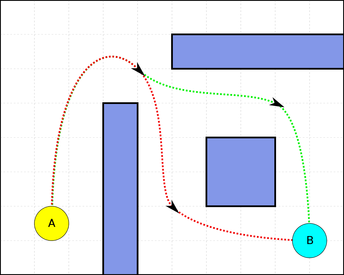
Two shortest paths between A and B

The fundamental problem of pathfinding is finding the shortest path between two points. Specifically, in pathfinding, we assume that we want to solve the problem for a single agent. Also, we assume that:

1. Time is discretized and actions can only be taken one at a time.
2. Actions are deterministic and durationless, i.e. applying an action is immediate and it would change the state by a deterministic function.
3. We have full knowledge about the world, i.e. where obstacles are located, how many points there are, etc.

Surely, there are other assumptions we make (i.e., the agents are cooperative and not self-interested). However, I aim to only explicitly write the assumptions that we will soon try to drop.

A classical algorithm in AI for solving the pathfinding problem is A*.  Given a weighted graph, A* maintains a tree of paths originating at the start node and extends those paths according to a heuristic one edge at a time until reaching the goal. If graphs, heuristics, and A* are new to you, follow the links for a great introduction for graphs and A*.

Generalizing to Multi-Agent Path Finding (MAPF)

A* solves the problem of single-agent pathfinding. But, in many real-world applications, we deal with multiple agents. Therefore, MAPF illustrates the problem of finding a shortest path for all agents to reach their goals without collisions (i.e., no couple of agents can be in the same location at the same time).

What do we mean by “shortest”?

For a single agent, we looked for the minimal number of actions it needs to perform to reach its goal. For multiple agents, there are two main metrics for path length in use today:

1. Sum Of Costs - As it sounds, simply sum the cost of all agents’ paths. 
2. Makespan - Take the maximal single-agent cost.

Clearly, optimizing for each metric will result in different shortest path solutions. I will focus on algorithms that optimize for the Sum Of Costs.

Exponential search-space

Fortunately, A* time complexity is polynomial (given a good heuristic). Generally, in computer science, a polynomial running time is considered efficient. Can we generalize it to multiple agents and keep the polynomial time complexity?

First, we need to remember about A* branching factor. The branching factor of a graph is the number of children at each node. For A* with a single agent, where the agent performs one action (out of b actions) at each time step, the branching factor is b. For A* with k agents, at each timestep we need to consider all possible actions (b) for all agents (k), leaving us with a branching factor of \(b^k\). For a simple grid-world with 5 possible actions (wait, or move right/left/up/down), the branching factor for 20 agents is 5²⁰ =95,367,431,640,625. Clearly, a trivial generalization of A* to MAPF is not feasible. Moreover, MAPF has already proven to be NP-Hard.

A* Improvements

So, how can we tackle that exponential branching factor? Back in 2010, Standley proposed a simple yet powerful idea - let’s try to divide the problems into smaller subproblems, and solve for each subproblem! Specifically, he proposed an iterative algorithm called Independence Detection (ID) which begins by searching for the shortest path for each agent alone and checking for conflicting agents. When a couple of conflicting agents are found, they are merged to be a group. This process of replanning and merging groups is repeated until there are no conflicts between the plans of all groups. Even though this algorithm hasn’t improved the worst-case time complexity of A*, it did, in fact, reduce the runtime to be exponential by the number of agents in the largest independent subproblem.

Yet, for problems with dependent groups consisting of only dozens of agents, we still have a very expensive search space to explore.

Therefore, Standley suggested modifying the search space. As we now know, at each timestep at \(A^*\), we generate nodes for all possible actions of all agents. Then, we expand the nodes with minimal f-value (sum of current path costs and heuristic prediction of future cost). Generated nodes with costs higher than the optimal cost are called surplus nodes. An important enhancement to A* would be to avoid generating surplus nodes.

Standley’s method to avoid the generation of surplus nodes is called Operator Decomposition (OD). OD suggests applying orders for the agents. When expanding a node, OD applies only the moves of the first agent, introducing an intermediate node. At intermediate nodes, only the moves of the next agent are considered, thus generating further intermediate nodes. When the last agent action is expanded, a regular node is generated.  So basically, Operator Decomposition trades tree width for depth, hoping that a good heuristic would allow it to avoid the generation of surplus nodes.

Another algorithm that tackles the surplus node generation problem is Enhanced Partial Expansion A* (EPEA*). Despite not explaining EPEA* here, it is important to note that practically it is shown that given a priori knowledge about the domain, EPEA* outperforms OD for the task of avoiding surplus node generation.

Moving to another space

All the above algorithms execute A* on the agent state space. Even though A* enhancements indeed improve the performance of the algorithm significantly, it is generally still very computationally expensive to solve for large maps with many agents (more than 100). Therefore, two MAPF algorithms developed over the last decade have tried to change the state space they search upon. Both can be viewed as two-level solvers.

Increasing Cost Tree Search (ICTS)

ICTS combines a high-level and low-level solver. The high-level solver searches the Increasing Cost Tree (ICT). At ICT, every node contains a vector of length k of costs allowed for each agent path. The ICT root node contains a vector with the cost of each agent’s shortest path length (without considering other agents). Then, the low-level solver’s job is to validate if a joint solution can be found by planning for each agent separately under the defined cost by the high-level solver. It is important to note that ICTS low-level solver doesn’t plan for the agents together, but rather only checks for conflicts between single-agent paths at a given cost.

If the low-level solver failed to find non-conflicting shortest paths under the given cost vector, the high-level solver expands the ICT root by generating k ICT nodes, where each node corresponds to increasing the cost for one of the agents by one. The high-level solver performs a breadth-first search of the ICT (which guarantees to find the optimal solution).

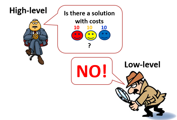
Illustration of ICTS algorithm for 3 agents. Taken from Roni Stern’s slides

For me, it felt weird that ICTS would work better, yet with a good implementation of the low-level solvers (using MDD) and pruning techniques for the ICT nodes, ICTS might outperform other optimal MAPF algorithms.

It is important to note that ICTS did not magically remove the exponential factor of the time complexity. It is still exponential, but to another factor - the ICT depth. Thus, intuitively, as the optimal solution single-agent path costs would be further away from the single-agent path costs when planned individually, the high-level solver would need to build a deeper ICT. The time complexity of ICTS is exponential by that depth.

Conflict Based Search (CBS)

CBS is also a two-level solver that searches in different state spaces. Specifically, it searches in conflict space.

CBS associates agents with constraints. A constraint is defined for a specific agent (a), a location (v) which he must avoid at a specific time step (t). A constraint is noted by a tuple (a, v, t).

For every single agent, CBS low-level solver searches for a shortest path that is consistent given a set of constraints. CBS high-level solver searches the constraint tree (CT). The CT is a binary tree, where each node contains a set of constraints and a solution consistent with the constraints (consistent means that all constraints are satisfied). The consistent solution is found by the low-level solver for every single agent. Then, CBS high-level solver checks for conflicts in the single-agent shortest paths. If no conflicts are found, we found the optimal plan. Yet, if a conflict is found, the high-level solver splits the corresponding CT node and generates nodes with constraints that avoid the conflict we found. Performing a best-first search on the CT is guaranteed to find the optimal solution.

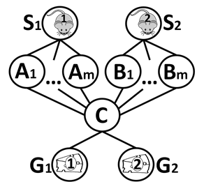
A canonical MAPF example. CBS will generate a node with a constraint for one of the mice at timestep 2 at location C, and will then find an optimal joint path.

During the 6 years since CBS was developed, it emerged as a powerful MAPF algorithm and was suggested with many improvements. The main weakness being addressed is its runtime being exponential to the number of conflicts it needs to solve. Thus, in crowded problems with many conflicts, it would perform poorly.

Reduce MAPF to another NP-Hard problem

Another interesting line of work for MAPF is by reduction to other NP-Hard problems. The idea behind it is that researchers have already developed powerful algorithms for other NP-Hard problems during the last decades. Therefore, instead of developing MAPF algorithms, we can just reduce MAPF and use existing solvers.

I won’t dive into the details of the reductions made, but I will state that this line of research has lately been shown to produce highly powerful MAPF algorithms. A partial list of the NP-Hard problems which successfully solve a reduction of MAPF contains Boolean Satisfiability (SAT), Mixed Integer Programming (MIP), Constraint Programming (CP).

So… What MAPF algorithm should I use?

Well, it depends. Basically, if you know the specific properties of your MAPF domain (Is it a large graph? How many agents? Are the agents crowded?), current research has some guidelines about what algorithm to use. Yet, selecting the most suitable algorithm for a MAPF problem is currently under research. Recently, a thorough analysis of the different MAPF algorithms had been made and points out cases where some algorithms are better than others.

Dynamic MAPF

An autonomous intersection model, where each car is an agent. The intersection aims to minimize the delay induced by the coordination between several agents.

The dynamic variant of MAPF extends it to be practical for a wide range of interesting practical problems (such as Autonomous Intersection Management). It is a highly interesting variation of MAPF. However, we focus on the “multi-agent path” from A* to MARL, and will not get into it. I encourage the curious reader to read the papers about online MAPF and lifelong MAPF.

Conclusion

We started from the basic problem of shortest pathfinding for a single agent and generalized it to the multi-agent pathfinding problem. We saw that even for that relatively “easy problem”, where we assumed full knowledge about the world, discretized time, and deterministic actions, finding an optimal solution is difficult and might be intractable. Then, we heard about the interesting generalization of MAPF to dynamic problems. Of course, there are many other interesting variants of MAPF, such as self-interested agents, yet I focused on the classical MAPF problem. Next, we will look at the generalized problem of AI planning, which is the case when our agents can do a little more than just move, and need to fulfill more complex goals. Then, we will continue to remove more and more assumptions, until we end up with Multi-Agent Reinforcement Learning.

Acknowledgment

I want to thank Roni Stern, my MSc thesis supervisor. My interest in this area and large parts of this blog series stems from the wonderful course he teaches on multi-agent systems at Ben-Gurion University, which I had the privilege to take.